Relative Volatility Index Variable MA (RVI-VMA) – Test Results

The Variable Moving Average (VMA) dynamically adjusts its own smoothing period to the changing market conditions based on a Volatility Index (VI).  While any VI can be used, in this article we will look at how the VMA performs using the Relative Volatility Index (RVI).

The RVI-VMA requires three user selected inputs: A Standard Deviation (SD) period, a Wilder’s Smoothing (WS) period and a VMA constant.  We tested trades going Long using Daily data taking End Of Day (EOD) signals~ analyzing all combinations of:

SD = 10, 20, 40, 80, 126, 252

WS = 9, 14, 19

VMA = 5, 10, 15, 20, 25, 30, 35, 40, 45, 50

The SD lengths were selected due to the fact that they correspond with the approximate number of trading days in standard calendar periods: 10 days = 2 weeks, 20 days = 1 month, 40 days = 2 months, 80 days = ⅓ year, 126 days = ½ year and there are 252 trading days in an average year.

The WS periods were selected because the standard setting for a RVI is 14 and it makes sense to test a few days either side of this in search of the best option.

The VMA periods were selected after preliminary tests showed that when combined with the different SD lengths they resulted in median smoothing periods between 3 and 173 days; a range that should capture the best results based on what we know from previous research into moving averages.

A total of 180 different averages were tested and each one was run through 300 years of data across 16 different global indexes (details here).

Download A FREE Spreadsheet With Raw Data For

All 180 RVI-VMA Long and Short Test Results

.

RVI Variable Moving Average EOD Returns, Long:

.RVI-VMA Annualized Return - Long, WS Period Comparison
.

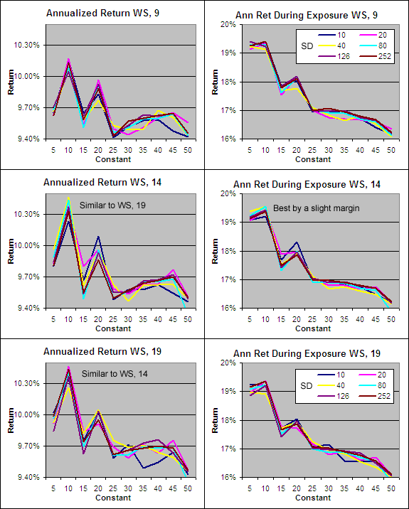
As with our previous VMA tests, every single RVI-VMA using EOD signals outperformed the average buy and hold annualized return of 6.32%^ during the test period (before allowing for transaction costs and slippage).

The charts above are split into three sets according to their WS period.  Each set reveals very similar results but, low and behold the standard setting of 14 proved the best by a small margin.

To our surprise the Standard Deviation period didn’t really matter and despite testing a huge range from 10 days to 252 days, all the results were very similar.  So we decided to select 126 days as the best SD period becuase it has been the best Volatility Index setting in several previous VMA tests.

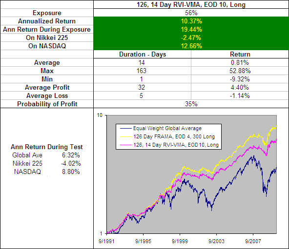
For the VMA constant, a period of 10 stood out as producing the best results across the board.  Therefore we want a RVI-VMA within a SD period of 126, a WS period of 14 and a VMA constant of 10:

.

Best EOD Relative Volatility Index Variable Moving Average:

.
126, 14 Day RVI-VMA, EOD 10, Long.

I have included on the above chart the performance of the 126 Day FRAMA, EOD 4, 300 Long becuase so far this has been the best performing Moving Average.  The 126, 14 Day RVI-VMA, EOD 10, Long can’t compare in terms of performance with the FRAMA and offers no outstanding attributes in any other areas.

.

126, 14 Day RVI-VMA, EOD 10 – Smoothing Period Distribution:

.
126 Day RVI-VMA, EOD 10 – Smoothing Period Distribution.

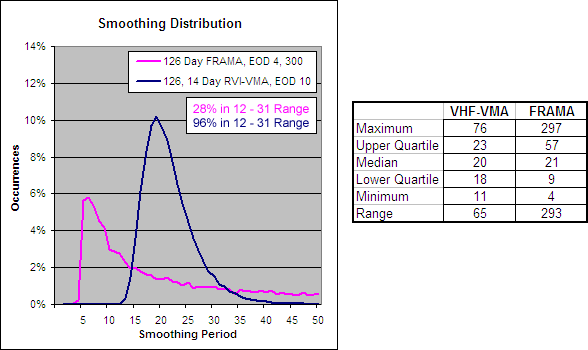
The RVI-VMA is very localized around its median smoothing period of 20.  Almost the entire distribution (96%) is covered with a 12 – 31 range which only represents 28% of the smoothing for the better performing FRAMA.

.

126, 14 Day RVI-VMA, 10 – Alpha Comparison

.

To get an idea of the readings that created these results we charted a section of the alpha for the 126, 14 Day RVI-VMA, 10 and compared it to the best performing FRAMA to see if there were any similarities that would reveal what makes a good volatility index:

.
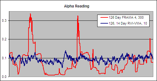
126 Day ER-VMA, 1 – Alpha Comparison.

As you can see the Alpha for the 126, 14 Day RVI-VMA, 10 is very volatile but stays within a tight range.  The better performing 126 Day FRAMA 4, 300 on the other hand produces readings that are much more stable however they do move to extremes upon occasion resulting in a more ‘Variable’ Moving Average.

.

Conclusion

.

The RVI-VMA outperformed a buy and hold approach in our tests but is nowhere neat as effective as the FRAMA and therefore is not worthy of being used as a trading tool.

Want to have a play with this indicator anyway?  Get a free Excel spreadsheet at the flowing link under Downloads – Technical Indicators: Variable Moving Average (VMA).  It will automatically adjust to one of many different VIs that you can select including the Relative Volatility Index featured in this article.

.

For more in this series see – Technical Indicator Fight for Supremacy

.

  • ~ An entry signal to go long for each average tested was generated with a close above that average and an exit signal was generated on each close below that moving average. No interest was earned while in cash and no allowance has been made for transaction costs or slippage. Trades were tested using End Of Day (EOD) signals on Daily data. Eg. Daily data with EOD signals requires the Daily price to close above a Daily Moving Average to open a long and vice versa.
  • ^ This was the average annualized return of the 16 markets during the testing period. The data used for these tests is included in the results spreadsheet and more details about our methodology can be found here.
Standard Deviation Ratio Variable Moving Ave (SDR-VMA) – Test Results

The Variable Moving Average (VMA) dynamically adjusts its own smoothing period to the changing market conditions based on a Volatility Index (VI).  While any VI can be used, in this article we will look at how the VMA performs using a Standard Deviation Ratio (SDR).  This is the VI that Tushar S. Chande first suggested be used when he presented what he called a Volatility Index Dynamic Average (VIDYA) in the March 1992 edition of Technical Analysis of Stocks & Commodities – Adapting Moving Averages To Market Volatility.

The SDR-VMA requires three user selected inputs: A Short Standard Deviation (SD1), a Longer Standard Deviation (SD2) and a VMA period.  We tested trades going Long and Short, using Daily data, taking End Of Day (EOD) and End Of Week (EOW) signals~ analyzing all combinations of:

SD1 = 10, 20, 40, 80, 126

SD2 = 20, 40, 80, 126, 252

VMA = 5, 10, 15, 20, 25, 30, 35, 40, 45, 50

The SD lengths were selected due to the fact that they correspond with the approximate number of trading days in standard calendar periods: 10 days = 2 weeks, 20 days = 1 month, 40 days = 2 months, 80 days = ⅓ year, 126 days = ½ year and there are 252 trading days in an average year.

The VMA periods were selected after preliminary tests showed that when combined with the different SDR combinations, these settings resulted in a median smoothing period between 6 and 280 days; a range that should capture the best results based on what we know from previous research into moving averages.

A total of 390 different averages were tested and each one was run through 300 years of data across 16 different global indexes (details here).

Download A FREE Spreadsheet With Raw Data For

All 390 SDR-VMA Long and Short Test Results

.

SDR Variable Moving Average Test Results, Daily EOD, Long:

.

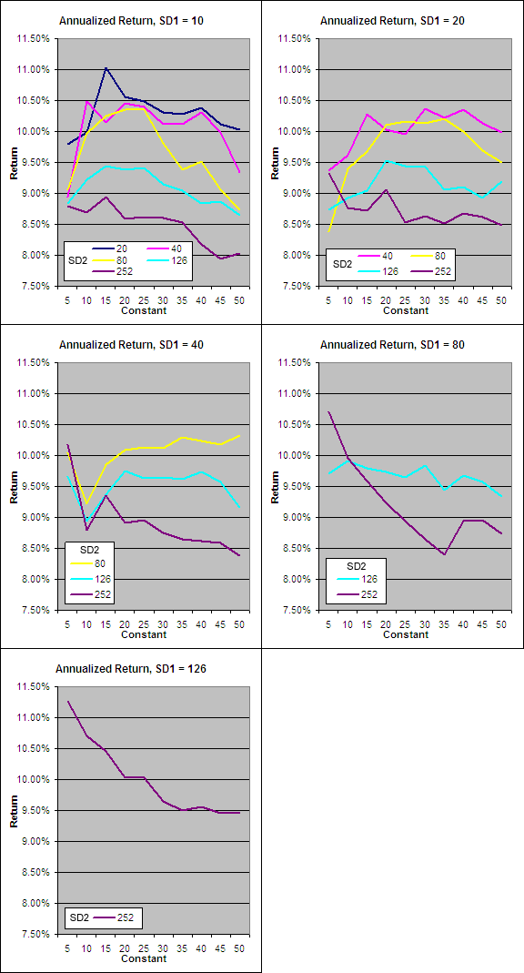
The data collected from our tests has been split by SD1 length with return plotted on the “y” axis, the VMA constant on the “x” axis and a separate series displayed for each SD2 length.

.

VIDYA Annualized Return.

First up it must be noted that every single SDR-VMA Long using EOD signals on Daily data outperformed the average buy and hold annualized return of 6.32%^ during the test period (before allowing for transaction costs and slippage).  This is a vote of confidence for the concept especially seeing as each average was typically sitting in cash 37% of the time.

Perhaps the most interesting information from the data however is the fact that the best performer from each set had a SD2 that was twice the length of SD1.  This formula of SD2 = 2*SD1 should therefore be used whenever utilizing the Standard Deviation Ratio.

.

The Best SDR-VMA Parameters

.

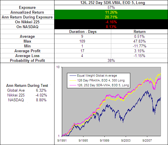
The best performing average was found where SD1 = 126, SD2 = 252 and the VMA constant = 5.  In the FRAMA tests we also saw that the periods of 126 (half a year) and 252 (a full trading year) produced the best results so this appears to be a reoccurring theme:

.

126, 252 Day SDR-VMA, EOD 5, Long.

I have included on the above chart the performance of the 126 Day FRAMA, EOD 4, 300 Long becuase so far this has been the best performing Moving Average and as you can see the SDR-VMA under performs.  To make matters worse it has an typical trade duration of just 9 days compared to the FRAMA’s 14, and underperformed the buy and hold returns of both the Nikkei 225 and the NASDAQ.  Therefore we can conclude that the SDR-VMA, despite being effective is not as good as the FRAMA.

.

A look at the Smoothing Period:

.

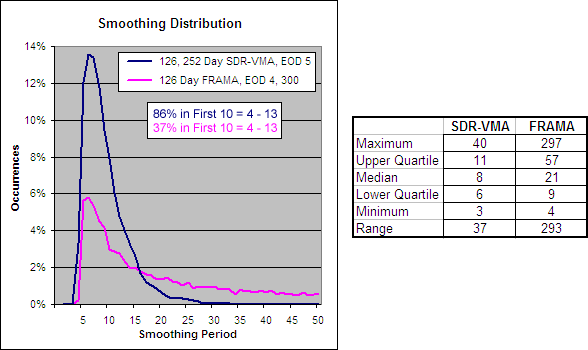
126, 252 Day SDR-VMA, EOD 5 - Smoothing Period Distribution.

By looking at the smoothing distribution you can see why the SDR-VMA is so much faster than the FRAMA.  While the FRAMA has a range of 293 days and a median of 21, the SDR-VMA has a range of just 37 days and a median of 8.

.

126, 252 Day SDR-VMA, 5 – Alpha Comparison

.

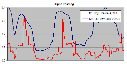
To get an idea of the readings that created these results we charted a section of the alpha for the 126, 252 Day SDR-VMA, 5 and compared it to the best performing FRAMA to see if there were any similarities that would reveal what makes a good volatility index:

.

126, 252 Day SDR-VMA, 5 - Alpha Comparison.

The alpha patterns are similar for both the 126 Day FRAMA 4, 300 and the 126, 252 Day SDR-VMA 5 but the readings are still very different.  The SDR-VMA’s indicator is nearly always higher than the FRAMA’s which is why the resulting VMA is much faster.

It is desirable to see however that the SDR-VMA’s alpha is so clean and noise free in its movements.  This leads me to believe that the 126, 252 SDR would be a good VI if it were adjusted to produce a slower average.  Also due to the lack of noise from the SDR it may offer value in other applications such a way of ranking a universe of stocks by their trend strength, but that is the topic of another set of tests.

.

For more in this series see – Technical Indicator Fight for Supremacy

.

  • ~ An entry signal to go long (or exit signal to cover a short) for each average tested was generated with a close above that average and an exit signal (or entry signal to go short) was generated on each close below that moving average. No interest was earned while in cash and no allowance has been made for transaction costs or slippage.  Trades were tested using End Of Day (EOD) and End Of Week (EOW) signals on Daily data.  Eg. Daily data with an EOW signal would require the Week to finish above a Daily Moving Average to open a long or close a short while Daily data with EOD signals would require the Daily price to close above a Daily Moving Average to open a long or close a short and vice versa.
  • ^ This was the average annualized return of the 16 markets during the testing period. The data used for these tests is included in the results spreadsheet and more details about our methodology can be found here.
Relative Volatility Index (RVI)

The Relative Volatility Index was created by Donald Dorsey and first presented in the June 1993 issue of Technical Analysis of Stocks and Commodities – The Relative Volatility Index.  He noticed that most technical analysts look for confirmation from several indicators before initiating a trade in order to reduce the occurrence of false signals.  This is a logical approach however many indicators are simply variations on the same calculation.  Dorsey described this as “not unlike taking two wind direction readings rather than reading the wind direction and barometric pressure to predict tomorrow’s weather”.

Because most indicators measure price change, Dorsey developed the RVI as a confirming indicator that measures the direction of volatility.  It is almost identical to the Relative Strength Index (RSI) but uses the standard deviation of high and low prices.

“There is no reason to expect the RVI to perform any better or worse than the RSI as an indicator in its own right.  The RVI’s advantage is as a confirming indicator because it provides a level of diversification missing in the RSI.”

How To Calculate the Relative Volatility Index

RVI = 100 * U / (U + D)

Where:

U = Wilder’s Smoothing,N of USD

D = Wilder’s Smoothing,N of DSD

USD = If close > close(1) then SD,S else 0

DSD = If close < close(1) then SD,S else 0

S = User selected period for the Standard Deviation of the close (Dorsey suggested 10).

N = User selected smoothing period (Dorsey suggested 14)

(Instead of using Wilder’s Smoothing we use an EMA with a period of (N*2)-1 which produces the same result but is faster to calculate.)

Here is an example of a RVI with an “S” and “N” of 3:

RVI Formula

Relative Volatility Index Excel File

I have put together an Excel Spreadsheet containing the Relative Volatility Index and made it available for FREE download.  It contains a ‘basic’ version displaying the example above and a ‘fancy’ one that will automatically adjust to the length you specify.  Find it at the following link near the bottom of the page under Downloads – Technical Indicators: Relative Volatility Index (RVI)


Relative Volatility Index Example

RVI Example

How to use the Relative Volatility Index

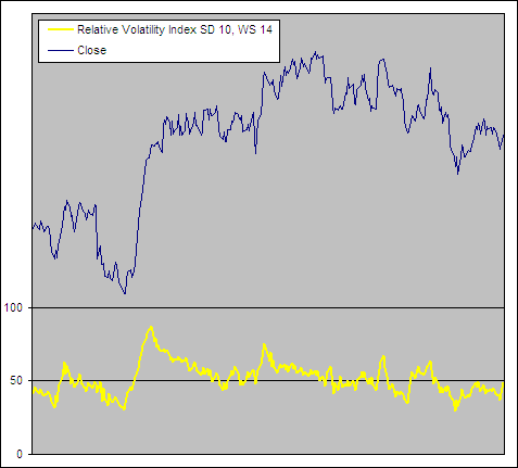
The Relative Volatility Index measures the direction and magnitude of volatility.  High readings indicate the market is moving up strongly, low readings indicate a strong bearish move and readings round 50 indicate a lack of direction.  In this way the RVI can be used to measure the strength or lack of a trend.  However like the RSI, extreme readings often warn of a reversal.

Here are the buy and sell rules that Dorsey developed for the RVI.  Keep in mind that he intended this as a confirming indicator not a stand alone system:

  • Buy only  if RVI > 50
  • Sell short only if RVI < 50
  • If you miss the first RVI buy signal buy when RVI > 60
  • If you miss the first RVI Sell signal sell when RVI < 40
  • Close a long position when the RVI falls below 40
  • Close a short position when the RVI rises above 60

In the September 1995 issue of Technical Analysis of Stocks and Commodities, Dorsey wrote a follow up article – Refining the Relative Volatility Index.  Here he presented the idea of using the average of two RVIs; one of high prices and one of low prices and then smoothing the result with a 20 day Linear Regression Indicator.  He called the new version “Inertia”.

“A trend is simply the outward result of inertia.  Once a market starts to move, it takes significantly more energy for it to change direction than for it to continue along the same path.”


In Physics Inertia is described as the amount of resistance that an object requires for a change in velocity.  To get a reading of Inertia requires a measure of mass and direction.  In the stock market there are many different ways (each of varying effectiveness) to measure direction but what about mass?

Because volatility reveals the markets propensity to make various sized movements regardless of direction, Dorsey saw it as a possible measure for mass.  If his theory is correct then the RVI should be a particularly useful trend indicator.

His modified version of the Relative Volatility Index or “Inertia” can be used as a long term trend indicator where readings above 50 indicate positive Inertia and readings below 50 indicate negative Inertia or a bearish trend.


Test Results

As part of the ‘Technical Indicator Fight for Supremacy‘ We have tested/will test the Relative Volatility Index as a component in several technical indicators:

We will also be testing its stand alone buy and sell signals and if they are good then we see how it performs as a confirming indicator.

Vertical Horizontal Filter (VHF)

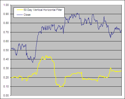
The Vertical Horizontal Filter (VHF) was first presented by Adam White in an article published in the August, 1991 issue of Futures Magazine – Tuning into trendiness with VHF indicator.  Trend following indicators work best in a trending market while in a range bound market, mean reversion strategies tend to excel.  The Vertical Horizontal Filter is designed to determine if prices are in a trending or congestion phase so that the most appropriate trading strategy can be applied.

The Vertical Horizontal Filter can be interpreted in several different ways:

  1. Values can be used to indicate the strength of the trend; higher values equal a stronger trend.
  2. The VHF direction can be used to identify if a trending or congestion phase is developing.
  3. It can also be used as a contrarian indicator where extreme readings foretell of an impending change in the market phase.

.

How To Calculate the Vertical Horizontal Filter:

.

VHF = Numerator / Denominator

Where:

Denominator = n ∑ (ABS(Close – Close[1]))

Numerator = ABS (Max Close[n] – Min Close[n])

n = Number of Periods

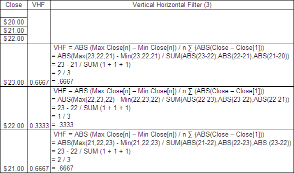
Here is an example of a 3 period VHF:

.

Vertical Horizontal Filter Formula.

Vertical Horizontal Filter Excel File

.

I have put together an Excel Spreadsheet containing the Vertical Horizontal Filter and made it available for FREE download.  It contains a ‘basic’ version displaying the example above and a ‘fancy’ one that will automatically adjust to the length you specify.  Find it at the following link near the bottom of the page under Downloads – Technical Indicators: Vertical Horizontal Filter (VHF)

.

Vertical Horizontal Filter Example

.

Vertical Horizontal Filter
.

Test Results

.
As part of the ‘Technical Indicator Fight for Supremacy‘ We have tested/will test the Vertical Horizontal Filter as a component in several technical indicators:

We will also be testing it for buy and sell signals in conjunction with trending and mean revision indicators.

.

Standard Deviation Ratio (SDR)

The Standard Deviation Ratio (SDR) was first presented as a technical indicator in the March 1992 edition of Technical Analysis of Stocks & Commodities magazine ‘Adapting Moving Averages To Market Volatility‘.  The author Tushar S. Chande, Ph.D. used it as the Volatility Index in the original version of his Volatility Index Dynamic Average (VIDYA) or Variable Moving Average (VMA).

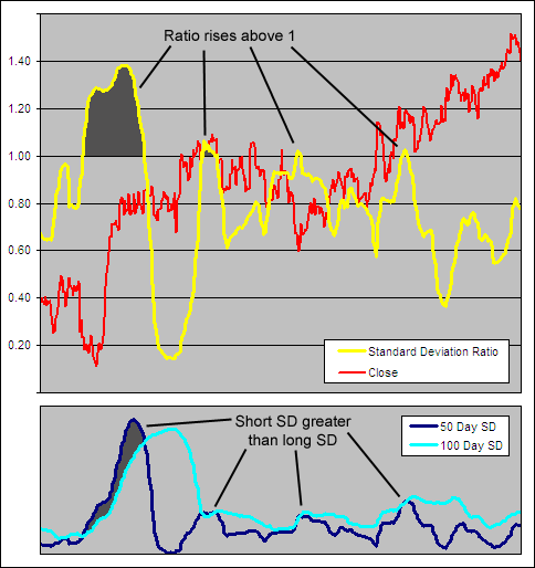
Calculating it is as simple as taking the ratio of a Standard Deviation (SD) over one period to that of a longer period where both have the same starting point.  One quirk of the SDR is that because the short term SD can become greater than the longer term SD, the ratio has no upper limit but does tend to remain below 1 most of the time (see the example chart below).  The higher the ratio, the more spread the recent data is from the mean in relation to the past which should indicate a stronger trend.

It is very helpful to know the strength or lack of a trend as different approaches will be more profitable depending on the market type.  But is the Standard Deviation Ratio an effective way to reveal the strength of a trend?  To find out we are entering it in the Technical Indicator Fight for Supremacy.  We will be testing the SDR as a component in the VIDYA, an Adaptive Moving Average and an Indicator Weighted Moving Average.

.

50 / 100 Standard Deviation Ratio Example

.

Standard Deviation Ratio

.

Standard Deviation Ratio Excel File

.

I have put together an Excel Spreadsheet containing the Standard Deviation Ratio and made it available for FREE download.  While the SDR may be very easy to calculate this spreadsheet will automatically adjust to the parameters you specify.  Find it at the following link near the bottom of the page under Downloads – Technical Indicators: Standard Deviation Ratio (SDR)

.

Test Results

.
As part of the ‘Technical Indicator Fight for Supremacy‘ We have tested/will test the Efficiency Ratio as a component in several technical indicators:

  • Standard Deviation Ratio Variable Moving Average (SDR-VMA) – Completed Results
  • Standard Deviation Ratio Adaptive Moving Average (SDR-AMA) – Completed Results
  • Standard Deviation Ratio Log Normal Adaptive Moving Average (SDR-LAMA)
  • Standard Deviation Ratio Weighted Moving Average (SDR-WMA)

We will also test the SDR as a filter, only taking trades when it indicates a strong trend.

Standard Deviation

Standard Deviation (SD) reveals how much a data set varies from its mean; a high Standard Deviation indicates that the data is widely spread.  With stock prices it can be used as a measure of the historical volatility to reveal the theoretical probability of a price change over a specified period.  This information can be used in many ways such as a measure of risk or as a component in technical indicators.

.

Normal Distribution Bell Curve

.

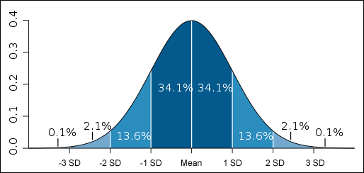
Normal Distribution - Bell Curve.

A data set that is Normally Distributed with produce a probability curve called a bell curve, like the one above.  One standard deviation from the mean accounts for 68% of the occurrences while two SDs covers 95% and three covers 99.7%.  One of the challenges with the stock market is that the data is not Normally Distributed but instead exhibits Fat Tails.  So the Standard Deviation is far from a perfect measure but is still a useful trading tool in some applications.

.

How To Calculate Standard Deviation

.

Standard deviation is the square root of variance and can easily be calculated in an Excel spread sheet with the =STDEVP() function or it can be done the hard way using the following formula:

.

Standard Deviation Formula

.

Where:

SMA = Simple Moving Average

N = Number of periods

.

Standard Deviation Example

.

If we take the percentage change of the Dow Jones Industrial Average for the 10 years from 2000 – 2010 we get the following values:

-6.17%,   -7.1%,   -16.76%,   25.32%,   3.15%,   -0.61%,   16.29%,   6.43%,   -33.84%,   18.82%

To find the SD we first find the mean (average):

(-6.17%  +   -7.1%  +  -16.76%  +  25.32%  +  3.15%  +  -0.61%  +  16.29%  +  6.43%  +  -33.84%  +  18.82%) / N

= 5.53% / 10

= 0.55%

We then calculate the deviation of each data point from the mean (= Data Point – Mean), square the result and find the sum:

-6.72%^2  +  -7.66%^2  +  -17.32%^2  +  24.77%^2  +  2.6%^2  +  -1.16%^2  +  15.73%^2  +  5.88%^2  +  -34.39%^2  +  18.27%^2

= 28.24%

Finally divide the result by N to find the average and take the square root to reveal the SD

= √(28.24% / 10)

= 16.8%

This means that in theory (assuming a normal distribution), based on ten years of the Dow’s annual price changes, about 68% of years the Dow will move up or down within 16.8% (one standard deviation).  While about 95% of years the Dow should finish up or down within 33.6% (two standard deviations).

What Does Standard Deviation Mean?
1. A measure of the dispersion of a set of data from its mean. The more spread apart the data, the higher the deviation. Standard deviation is calculated as the square root of variance.

2. In finance, standard deviation is applied to the annual rate of return of an investment to measure the investment’s volatility. Standard deviation is also known as historical volatility and is used by investors as a gauge for the amount of expected volatility.

Investopedia Says

Investopedia explains Standard Deviation
Standard deviation is a statistical measurement that sheds light on historical volatility. For example, a volatile stock will have a high standard deviation while the deviation of a stable blue chip stock will be lower.

Double (D-EMA) and Triple Exponential Moving Average (T-EMA)

The Double and Triple Exponential Moving Average were created by Patrick Mulloy and first published in the February 1994 issue of Technical Analysis of Stocks & Commodities magazine – Smoothing Data With Less Lag.  Mulloy stated in his article:

.

“Moving averages have a detrimental lag time that increases as the moving average length increases.  The solution is a modified version of exponential smoothing with less lag time.”

.

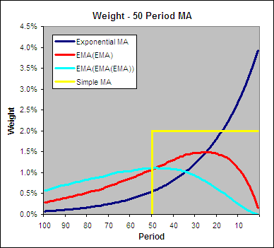
Like an EMA, the D-EMA and T-EMA apply more weight to the most recent data in an attempt to smooth out noise while still remaining highly reactive to changes in the data.  This is not achieved by simply double and triple smoothing as one may assume.  To do so results in weighting that resembles a backwards log-normal distribution, rather like a Triangular Moving Average but smooth and shifted forward.  Below you can see how the weighting is allocated by a single, double and triple smoothed exponential moving average compared to a standard EMA and SMA:

.

Double and Tripple Smoothed EMA Weighting.

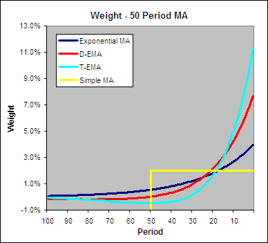
As you can see by double and triple smoothing an EMA the weighting no longer focuses on the latest data.  The actual Double and Triple Exponential Moving Average applies the weighing very heavily to the most recent data as illustrated in the chart below:

.

Double and Tripple EMA Weight

.

How To Calculate a Double Exponential Moving Average and T-EMA

.

Double Exponential MA Formula:

D-EMA = 2*EMA – EMA(EMA)

Triple Exponential MA Formula:

T-EMA = (3*EMA – 3*EMA(EMA)) + EMA(EMA(EMA))

Where:

EMA = EMA(1) + α * (Close – EMA(1))

α = 2 / (N + 1)

N = The smoothing period.

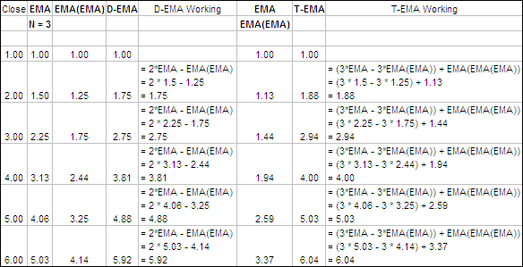
Here is an example of a 3 period Double Exponential Moving Average and Triple EMA:

.

Double and Triple Exponential Moving Average Formula.

Triple Exponential Moving Average and D-EMA Excel File

.

We have built a spreadsheet to calculate the D-EMA and T-EMA and have made it available for free download.  Find the file at the following link near the bottom of the page under Downloads – Technical Indicators: Double (D-EMA) and Triple Exponential Moving Average (T-EMA).

.

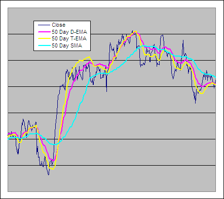
Double EMA, Triple EMA and a Simple Moving Average

.

Double and Tripple EMA Vs a Simple MA.


Double and Triple Exponential Moving Average Test Results


We ran them through tests through over 300 years of data across 16 different global markets.  Here are the results:

Double Exponential Moving average Vs Simple and Exponential Moving average


Double Vs Triple Exponential Moving Average


More in this series:

We have conducted and continue to conduct extensive tests on a variety of technical indicators.  See how they perform and which reveal themselves as the best in the Technical Indicator Fight for Supremacy.


Triangular Simple Moving Average (TriS-MA)

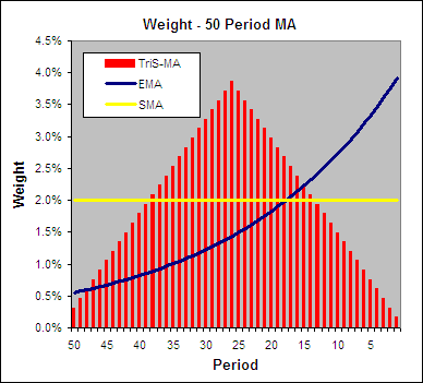
The Triangular Simple Moving Average (TriS-MA) is almost identical to the Triangular Weighted Moving Average but is very different in how it is calculated.  Instead of weighting the data points directly it is a double smoothed simple moving average (a moving average of a moving average).  Because most of the weight ends up being placed on the data in the middle of a series the weighting looks like a triangle, hence the name.  Below you can see how the weighting is applied to a 50 period TriS-MA, EMA and SMA:

.

Triangular Simple MA vs SMA and EMA Weighting.

How To Calculate a Triangular Simple Moving Average

.

TriS-MA = SUM(MA1,L) / L

Where:

MA1 = SUM(CLOSE,L) / L

L = ceiling((n+1) / 2)

n = Number of Periods

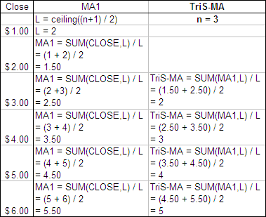
Here is an example of a 3 period Triangular Weighted Moving Average:

.

How to Calculate a Triangular Simple Moving Average

.

Triangular Simple Moving Average Excel File

.

An Excel Spreadsheet containing a Triangular Weighted Moving Average is available for FREE download.  It contains the ‘basic’ version you can see above and a ‘fancy’ one that will automatically adjust to the length you specify.  Find it at the following link near the bottom of the page under Downloads – Technical Indicators: Triangular Weighted Moving Average (TriW-MA).  Please let us know if you find it useful.

.

Triangular Moving Average and a Simple Moving Average

.

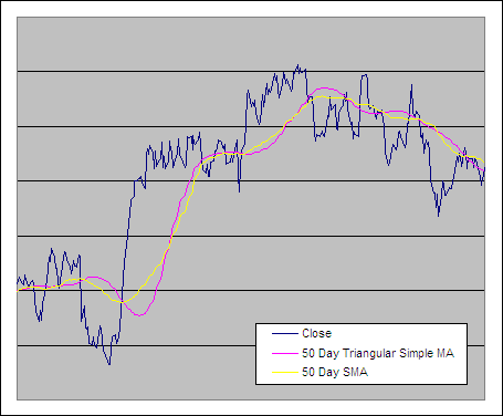
50 Day Triangular Simple MA and Simple MA.

Test Results

.

We tested several different types of Moving Averages including the TriS-MA through 300 years of data across 16 global markets to reveal which is the best and if any of them are worth using in your trading – see the results.

.

Exponential Moving Average (EMA)

The Exponential Moving Average (EMA) is a very popular method for smoothing data in an attempt to eliminate noise and our tests show that it is also highly effective.  Unlike the Simple Moving Average (SMA) that applies equal weight to all data, the EMA applies more weight to the recent data so that it reacts faster to sudden changes.

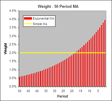
You can see see why it is called an Exponential Moving Average when you look at how the weighting is applied; it is in the shape of an exponential curve.  Because of this the weighting never reaches zero and the influence of early data always remains (although it has little effect outside of the specified smoothing period).  This is more clearly illustrated by the chart below which shows the weighting for a 50 period EMA and a SMA:

.

Weighting - Exponential Moving Average and a SMA.

Although we call it a 50 period EMA, those 50 periods only actually account for 86% of the weighting.  A further 12% is applied over the preceding 50 periods leaving the last 2% to be spread amongst all the prior data.  Here is a great article from MarketSci on this topic: Visual Depiction of SMA vs EMA Weighting

.

How To Calculate an Exponential Moving Average

.

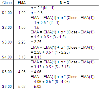
Calculating an Exponential Moving Average actually requires less processing power than a Simple Moving Average because it only refers to the current period and the previous EMA value.  While it does not become active until the Nth period the EMA starts with the first close price and after that is calculated according to the following formula:

EMA = EMA(1) + α * (Close – EMA(1))

Where:

α = 2 / (N + 1)

N = The smoothing period.

Here is an example of a 3 period Exponential Moving Average:

.

How to Calculate an Exponential Moving Average

If you have two data sets and you wish to find out the EMA smoothing period, the following formula will reveal it:

N = (2-( (MA-MA[1]) / (Close-MA[1]) ) ) / ( (MA-MA[1]) / (Close-MA[1]) )

.

Exponential Moving Average Excel File

.

The EMA is so simple to calculate that it is unlikely that you would need a version in Excel but we have put together one for those of you that are lazy :).  It is free and contains the ‘basic’ version you can see above and one that will automatically adjust to the length you specify.  Find it at the following link near the bottom of the page under Downloads – Technical Indicators: Exponential Moving Average (EMA).

.

Exponential Moving Average and a Simple Moving Average

.

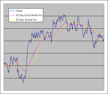
Exponential Moving Average vs Simple MA.

Test Results

.

If you haven’t already then check out the EMA test results.  We tested it against the SMA and D-EMA through 300 years of data across 16 global markets to reveal which is the best and the characteristics they exhibit as their smoothing period is changed.  See the results; Moving Averages – Simple vs Exponential

.

Linear Regression Indicator (LRI) & Time Series Forecast (TSF)

Linear Regression is a statistical tool used to predict future values from past values.  By using the least squares method, a straight line can be plotted that minimizes the distance between the resulting line and the data set in order to reveal a trend.

The Linear Regression Indicator (LRI) plots the end value of a Linear Regression Line at each data point.  A variation on the same idea is the Time Series forecast (TSF) which is found by adding the Linear Regression Slope to the Linear Regression Line.  The TSF basically projects the LRI forward one period.  The TSF is also sometimes referred to as a Moving Linear Regression or Regression Oscillator.

By calculating these two indicators on a moving basis the result looks similar to that of a moving average and can be used in the same way.

.

Calculating a Linear Regression Line

.

Linear Regression Line = a + bx

Where:

a = (Σy – bΣx) / n

b = (nΣ(xy) – (Σx) (Σy)) / (nΣx² – (Σx)²)

b = Linear Regression Slope.

x = The current time period.

y = The data series (Usually the close price).

n = Number of periods.

.

Linear Regression Indicator & Time Series Forecast Excel File

.

Calculating these indicators by hand is a pain in the ass so we have build an Excel spreadsheet containing both the Linear Regression Indicator and Time Series forecast that you can download for free.  Find it at the following link near the bottom of the page under Downloads – Technical Indicators: Linear Regression Indicator (LRI) & Time Series Forecast (TSF).  Please let us know if you find it useful.

.

Linear Regression Indicator, Time Series Forecast and a Simple Moving Average

.

Linear Regression Indicator, Time Series Forecast and SMA.

Test Results

.

We tested the Linear Regression Indicator and Time Series forecast through 300 years of data across 16 global markets to reveal which is the best and if either of them are worth using as trading tool for data smoothing – see the results.

.

.

Wilder’s Smoothing was developed buy J. Welles Wilder, Jr. and he used it as a component in several of his other indicators including the RSI which is one of the most popular technical indicators of all time.