Log-Normal Adaptive Moving Average (LAMA)

The Log-Normal Moving Average (LAMA) is the name I have given to an Adaptive Moving Average that uses the adaptive process developed by John F Ehlers for use in his FRAMA.  Stock prices are said to be Log-Normal so Ehlers used EXP to relate his Volatility Index (The Fractal Dimension) to Alpha.  The LAMA is designed so that any VI can easily be incorporated as long as it shifts between a range of 1 – 0 where high readings indicate high volatility.

How to Calculate an Log-Normal Moving Average

Seed it with the Close price then after that the LAMA is calculated according to the following formula:

LAMA = LAMA(1) + New α * (Close – LAMA(1))

Where:

New α = 2 / (New N + 1)

New N = ((SC – FC) * ((N – 1) / (SC – 1))) + FC

SC = Your choice of a Slow moving average > FC

FC = Your choice of a Fast moving average < SC

N = (2 – α) / α

α = EXP(W * (1 – VI))

W = LN(2 / (SC + 1))


***If the above formula does not make a lot of sense to you and you would like a more in depth explanation then please read this article on the Fractal Adaptive Moving average.


Log-Normal Adaptive Moving Average Excel File

I have put together an Excel Spreadsheet containing the Log-Normal Adaptive Moving Average and made it available for FREE download.  It contains a ‘basic’ version that shows all the working for the formula and a ‘fancy’ one that will automatically adjust to the length as well as the Volatility Index you specify.  Find it at the following link near the bottom of the page under Downloads – Technical Indicators: Log-Normal Adaptive Moving Average (LAMA)


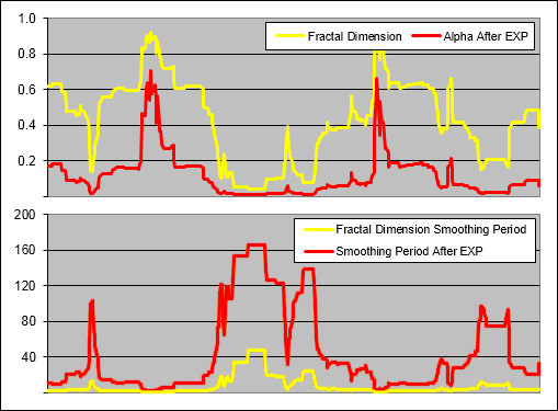
How EXP affects Alpha and the Smoothing Period:

Ehlers used EXP to relate the Volatility Index (VI) to Alpha (α) so lets have a look at what affect this has:

LNMA - EXP Affect on Alpha and SmoothingLNMA - EXP Affect on Alpha and Smoothing.

In the top chart you can see Alpha taken directly from the the Fractal Dimension and also taken after it has been modified by applying EXP.  In the bottom chart you can see the smoothing period that results from each version of Alpha.  Clearly by applying EXP, Alpha is reduced creating an significantly faster Smoothing Period.

The use of EXP results in not just a slower LAMA overall but one that exponentially slows as alpha decreases.  This affect is similar to that of raising Alpha to a power as seen in the Adaptive Moving Average (AMA).  In fact, it turns out that the LAMA is identical to the AMA if you were to raise it to the power of about 988,869,997.798!!!!!!  That is not a typo.  The LAMA and therefore the FRAMA is identical to the AMA raised the power of almost 100 million….

In discovering this there is little point in running the tests on this indicator because previous tests on the AMA already reveal it will not be able to out perform.  Oh well, that saves some work!  That is why we take the time to look closer at these things and try not to make too many uneducated assumptions.


More in this series:

We have conducted and continue to conduct extensive tests on a variety of technical indicators.  See how they perform and which reveal themselves as the best in the Technical Indicator Fight for Supremacy.


Adaptive Moving Average (AMA) aka Kaufman Adaptive Moving Average (KAMA)

The Adaptive Moving Average (AMA) aka Kaufman Adaptive Moving Average (KAMA) was created by Perry Kaufman and first presented in his book Smarter Trading (1995).  This moving average offered a significant advantage over previous attempts at ‘intelligent’ averages because it allowed the user greater control.

The Variable Moving Average – VMA (1992) for instance offered no upper or lower limit to its smoothing period.  The AMA on the other hand allowed the user to define the range across which they desired the smoothing to be spread.

It follows the same theory as the VMA in that depending on the market environment there will be different amounts of noise and therefore a different moving average speed will be required to achieve the most profitable results.  In a strongly trending market for instance, the noise levels are low and a faster moving average should produce the best results.  Conversely in a crab or sideways market the noise levels are very high and a slower average is likely to be better suited.

.

How to Calculate an Adaptive Moving Average

.

It starts with the Close price.

AMA(1) = Close

After that AMA is calculated according to the following formula:

AMA = AMA(1) + α * (Close – AMA(1))

You will notice that this is the same as the formula for an Exponential Moving Average (EMA):

EMA = EMA(1) + α * (Close – EMA(1))

But Alpha in an EMA is α = 2 / (N + 1) so it remains constant while for an AMA the Alpha is adaptive:

α = [(VI * (FC – SC)) + SC] ²

Where:

VI = Users choice of a measure of volatility or trend strength, Kaufman suggested his Efficiency Ratio (ER).

SC = 2 / (SN + 1)

SN = Your choice of a Slow moving average > FN

FC = 2 / (FN + 1)

FN = Your choice of a Slow moving average < SN

Here is an example of a 3 period AMA with a 3 period Efficiency Ratio (ER) as the VI:

.

Adaptive Moving Average Formula.

How Squaring Alpha affects the AMA Smoothing Range

.

Kaufman suggest that his AMA have a FC of 2 and a SC of 30 which would lead one to assume that the adaptive smoothing would be in the 2 – 30 range but you would be wrong because the alpha is squared.  For example, lets set the VI to zero so we can reveal the slowest possible average:

.

AMA Alpha Calculations.

Now to reveal the EMA smoothing period ‘N’ from alpha:

N (EMA) = (2 – α) / α
N (EMA) = (2 – 0.0042) / 0.0042
N (EMA) = 480

So in reality an AMA with a SN of 30 where alpha is raised to the power of 2 can actually move as slowly as a 480 day EMA.  Now to me that is not very user friendly; entering a parameter of 30 that results in a smoothing period of 480.  So I use the following formula for SC and FC instead:

SC = α(1)^(1/P)

Where:

α(1) = 2 / (SN+1)

P = Power that alpha is raised to (usually 2)

SN = Your choice of a Slow moving average > FN

Now SN will be the actual resulting slowest moving average even if you change the power that alpha is raised to.  I also use the same process for FN and FC.  Lets look again at Alpha with the VI set to zero, the FN at 2 and the SN at 480:

.

AMA New Alpha Calculations.

Now when we reveal the EMA smoothing period ‘N’ from alpha it should equal our user defined 480:

N (EMA) = (2 – α) / α
N (EMA) = (2 – 0.0042) / 0.0042
N (EMA) = 480

.

A closer look at the affect of Squaring Alpha

.

Understanding the affect of squaring alpha is very important as the chart below illustrates:

.

AMA Exponent Affect on Smoothing

.

As you can see above, an input smoothing period of 300 with alpha squared results in an actual smoothing period of over 45,300 which is totally useless.  However this is a setting that one could easily use without a proper understanding of how the AMA works.  In our testing we will be trying the AMA with alpha raised to powers other that 2 so some other examples have also been plotted on the chart above.

Below we look at the affect on alpha and the smoothing resulting from an AMA with the Efficiency Ratio taken directly into alpha (^1) or being squared (^2):

.

AMA - Alpha and Smoothing with and without Squaring

.

We used our modified AMA formula for the above charts so that the actual FN and SN were identically matched despite modifications to alpha.  As you can see, squaring alpha results in not just a slower AMA overall but one that is much faster to slow down when the alpha decreases.  Kaufman obviously wanted the AMA to very rapidly slow when the data lacked a trend.  This affect is similar to that of increasing the constant ‘N’ in the Variable Moving Average.

.

Is the AMA a Good Indicator?

.

As part of the ‘Technical Indicator Fight for Supremacy‘ we will be putting the AMA against several different types of moving averages and will test several different Volatility Indexes as components including:

We will also be testing the assumption that squaring alpha was a good idea and will try raising it to several different powers.

Can you think of any other worthwhile tests?  Please let us know in the comments section at the bottom.

.

Adaptive Moving Average Excel File

.

I have put together an Excel Spreadsheet containing the Adaptive Moving Average and made it available for FREE download.  It contains a ‘basic’ version that shows all the working and a ‘fancy’ one that will automatically adjust to the length as well as the Volatility Index you specify.  Find it at the following link near the bottom of the page under Downloads – Technical Indicators: Adaptive Moving Average (AMA)

.

Adaptive Moving Average Example, VI = 50 Day Efficiency Ratio

.

Kaufman Adaptive Moving Average vs EMA - Example

Weighted Moving Average (W-MA)

The Weighted Moving Average is going up against several other MAs in the ‘Technical Indicator – Fight for Supremacy‘ so lets briefly cover how it is calculated and to make things easy I have put together an Excel Spreadsheet for free download.

In an attempt to be more reactive to price changes a Weighted Moving Average applies the most weight to the latest data rather like an EMA does.  But instead of the weighting being exponential it is linear like a SMA.  Below you can see how the weighting is applied to a 50 period W-MA, EMA and SMA:

.

Weight - WMA vs EMA vs SMA.

How To Calculate a Weighted Moving Average

.

The Formula is:

W-MA = (PRICE*n + PRICE(1)*n-1 + … PRICE(n-1)*1) / (n * (n+1) / 2)

Where:

n = The smoothing period.

Here is an example of a 3 period Weighted Moving Average:

.

Calculating a Weighted Moving Average.

Weighted Moving Average Excel File

.

I have put together an Excel Spreadsheet containing a Weighted Moving Average and made it available for FREE download.  It contains a ‘basic’ version displaying the example above and a ‘fancy’ one that will automatically adjust to the length you specify.  Find it at the following link near the bottom of the page under Downloads – Technical Indicators: Weighted Moving Average (W-MA).  Please let me know if you find it useful.

.

Weighted Moving Average and a Simple Moving Average

.

Weighted Moving Average and a Simple MA

.

Test Results

.

We tested several different types of Weighted Moving Averages including the W-MA through 300 years of data across 16 global markets to reveal which is the best and if any of them are worthy of use as a trading tool.  See the results – Weighted Moving Averages Put To The Test

.

.

Wilder’s Smoothing was developed buy J. Welles Wilder, Jr. and he used it as a component in several of his other indicators including the RSI which is one of the most popular technical indicators of all time.

Wilder’s Smoothing AKA Smoothed MA (WS-MA)

Wilder’s Smoothing AKA Smoothed Moving Average is to duke it out in the ‘Technical Indicator – Fight for Supremacy‘ so here is some info about how it is calculated along with an Excel Spreadsheet for your interest:

Wilder’s Smoothing (WS-MA) was developed buy J. Welles Wilder, Jr. and first presented in his landmark book New Concepts in Technical Trading Systems (June 1978).  He used it as a component in several of his other indicators including the RSI which is one of the most popular technical indicators of all time.

Despite being very different in how they are calculated, Wilder’s Smoothing and the EMA are actually the same indicator.  To reveal the equivalent EMA simply multiply the period by two and subtract one, test it for yourself; a 50 period WS-MA is equivalent to a 99 period EMA.  You can also reveal the EMA smoothing period from any two data sets using the following formula:

N = (2-( (MA-MA[1]) / (Close-MA[1]) ) ) / ( (MA-MA[1]) / (Close-MA[1]) )

Below you can see how the weighting is applied to a 50 period WS-MA, EMA and SMA:

.

Wilder's Smoothing vs SMA vs EMA Weighting.

How To Calculate Wilder’s Smoothing:

.

It starts as a Simple Moving Average (SMA):

WSMA1 = Simple MA = SUM(CLOSE, N)/N

After that it is calculated according to the following formula:

WSMA(i) = (SUM1-WSMA1+CLOSE(i))/N

Where:

WSMA1 = Wilder’s Smoothing for the first period.

WSMA(i) = Wilder’s Smoothing of the current period (except for the first one).

CLOSE(i) = The current closing price.

N = The smoothing period.

Here is an example of a 3 period Wilder’s Smoothing AKA Smoothed Moving Average:

.

Who to Calculate Wilder's Smoothing.

Wilder’s Smoothing Excel File

.

I have put together an Excel Spreadsheet containing Wilder’s Smoothing and made it available for FREE download.  It contains a ‘basic’ version displaying the example above and a ‘fancy’ one that will automatically adjust to the length you specify.  Find it at the following link near the bottom of the page under Downloads – Technical Indicators: Wilder’s Smoothing (WS-MA).

.

Smoothed Moving Average and a Simple Moving Average

.

Wilder's Smoothing vs Simple Moving Average

.

Test Results

.

We tested Wilder’s Smoothing through 300 years of data across 16 global markets to reveal if it is an effective trading tool – see the results.

.

.

Wilder’s Smoothing was developed buy J. Welles Wilder, Jr. and he used it as a component in several of his other indicators including the RSI which is one of the most popular technical indicators of all time.