The Variable Moving Average (VMA) aka Volatility Index Dynamic Average (VIDYA) was developed by Tushar S. Chande and first presented in the March 1992 edition of Technical Analysis of Stocks & Commodities – Adapting Moving Averages To Market Volatility
Chande’s theory was that the performance of an exponential moving average could be improved by using a Volatility Index (VI) to adjust the smoothing period as market conditions change. The idea being that when prices are congested an average should slow down to avoid whipsaws but when prices are trending strongly an average should speed up to capture the major price moves.
He was not the first person to think along these lines; George R. Arrington, Ph.D introduced a variable Simple Moving Average based on Standard Deviation in the June 1991 edition of Technical Analysis of Stocks & Commodities – Building a Variable-Length Moving Average (VLMA). The YIDYA however represented a massive step forward from the VLMA because it allowed a much larger spread of smoothing periods.
.
How To Calculate a Variable Moving Average
.
VMA = (α * VI * Close) + ((1 – ( α * VI )) * VMA[1])
Where:
α = 2 / (N + 1)
VI = Users choice of a measure of volatility or trend strength.
N = User selected constant smoothing period.
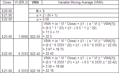
Here is an example of a 3 period VMA with a 3 period Efficiency Ratio (ER) as the VI:
.
 .
.
How the VIDYA Smoothing is changed by the Volatility Index
.
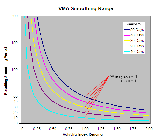
The Variable Moving Average is unique in that it has no upper or lower limit to its smoothing period:
.

.
The VMA smoothing period can go infinitely high until the Volatility Index equals zero at which point the resulting average will stop moving and be equal to the previous VMA. When the Volatility Index equals 1 the smoothing period will be equal to the user selected constant ‘N’; notice how when the Y axis = N, the X axis = 1.
However if the Volatility Index being used can rise above 1 (such as the Standard Deviation Ratio) then the smoothing period can drop below the user selected constant. When the VI = (N/2) + 0.5 then the smoothing period will be 1, which is equal to the price itself. Therefore the VI that is used must not rise above (N/2) + 0.5 and if it does upon occasion then this cap must be written into the formula.
.
A Look at the Actual Alpha
.
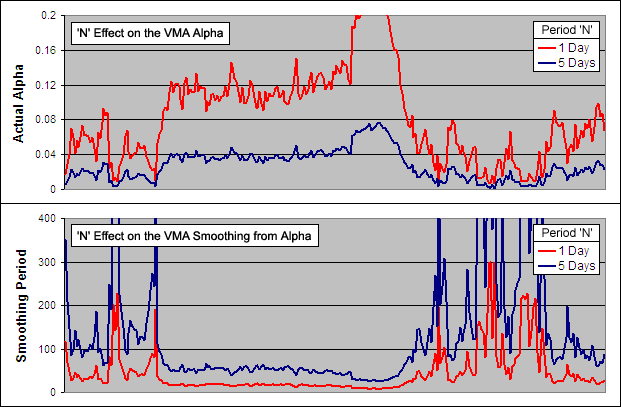
Because the VMA is as the name suggests, variable, the ‘Actual Alpha’ is not static but is influenced by the VI. By changing the constant ‘N’ however the interpretation of the VI changes greatly:
.
 .
.
Above you can see an example of the ‘Actual Alpha’ and the resulting smoothing period for a VMA with an ‘N’ of 1 and an ‘N’ of 5. We know that when the VI = 1 (indicating that the stock is trending perfectly) the smoothing period = ‘N’. So the fastest possible smoothing periods in these examples would be 1 and 5 respectively; not a big difference. But it is surprising to see what a huge impact changing ‘N’ just a few points has overall. In fact as ‘N’ increases the resulting VMA moves exponentially slower. This affect is rather like the squaring used by Kaufman in his Adaptive Moving Average.
.
What Volatility Index to use?
.
Chande originally used the Standard Deviation Ratio as his VI and this is the one typically used when people talk about a VIDYA. But later on, in the October 1995 article from Technical Analysis of Stocks & Commodities – ‘Identifying Powerful Breakouts Early‘ he suggested the use of his own Chande Momentum Oscillator (CMO).
Because the CMO ranges between 100 and -100, to use it in this application we must take the absolute value divided by 100. The result is identical to the Efficiency Ratio (ER) and is the VI used most often when people refer to a VMA. Any measure of volatility or trend strength can be used however as long as it fits between a zero to (N/2) + 0.5 range where higher readings indicate a stronger trend.
.
Volatility Indexes Used for Testing
.
As part of the ‘Technical Indicator Fight for Supremacy‘ we have tested/will test the following indicators as the Volatility Index in a Variable Moving Average:
- Standard Deviation Ratio (SDR) – Completed – Results
- Kaufman’s Efficiency Ratio (ER) – Completed – Results
- Relative Volatility Index (RVI) = RVI/100 – Completed – Results
- Vertical Horizontal Filter (VHF) – Completed – Results
- Fractal Dimension (D) = ABS(D – 2) – Completed – Results
- Chaikin’s Volatility (CV) * We currently lack High and Low Prices for some test markets.
Are there any others that you think are worth testing? Please let us know in the comments section at the bottom.
.
Variable Moving Average Excel File
.
I have put together an Excel Spreadsheet containing the Variable Moving Average and made it available for FREE download. It contains a ‘basic’ version that shows all the working and a ‘fancy’ one that will automatically adjust to the length as well as the Volatility Index you specify. Find it at the following link near the bottom of the page under Downloads – Technical Indicators: Variable Moving Average (VMA)
.
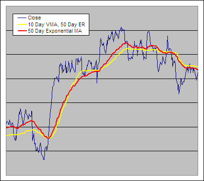
10 Day Variable Moving Average Example, VI = 50 Day Efficiency Ratio
.

bookmarking to read when my caffeine intake is a little higher
Hey Steve,
Just checked out your site http://www.investingwithoptions.com/. Nice to see another young trader making it happen. Yes guilty of writing some rather heavy posts.
Cheers
Derry
yeah i tried to explain heteroskedacity at 7 AM this morning, that did not go well
Thanks Brother this is great ! the explanation of the math behind it is very helpful 🙂
now that i understand how each parts of the equation works i can play with it 🙂
one question… VMA[1] for the fist data point you just use the Close[1]? and in that case why not just use Close[1] it should be more responsive to price change
I do have to agree with steveplace, heteroskedacity is hard to explain at 7:00 in the morning lol
dr.B
Glad that you found it useful Peter. I find some of the formulas around the web for these things really difficult to read because I don’t have any formal math education. That is why I break it all down and show the working so there is no confusion.
With regards to your question; the VMA is still an exponential moving average (EMA) http://etfhq.com/blog/2010/11/08/exponential-moving-average/ but with a dynamic alpha instead of a constant one. All EMAs use their previous average as they move forward but need to be seeded with a number at the start (usually the previous close) EMA = EMA(1) + α * (Close – EMA(1)). If you continued to use the previous close then the average would track the price so closely as to match it almost exactly.
Download the spread sheet if you haven’t already and have a try. Go to cell J5 at the end of the formula it will say IF(J4″”,J4+(2/(I5+1))*($E5-J4),””)) change this to read IF(E4″”,E4+(2/(I5+1))*($E5-E4),””)) fill this formula to the bottom of the column and it will then reference the previous close instead of the previous VMA.
BTW I just noticed that I had the spreadsheet set to manual calculation update rather than automatic. You may want to change this or download it again as I have fixed it now.
Cheers
Derry
i am using VMA along with other MA’s (simple, exp, weighted, vol weighted,triangular).
should i use the same period for VMA as the period for other averages?
do i use intersection as my buy/sell points as other MA’s? or
should i use the direction of VMA as my buy/sell signal?
thanks for your support.
Hi Sayyed,
You can see test results for several of the MAs you mentioned here – http://etfhq.com/blog/2010/05/25/best-technical-indicators/
The answer to your question depends on whether you are using them as part of a mechanical system or a discretionary one. I have not tested the results of MA crossovers between different types of MAs but I wouldn’t expect this to be an effective approach.
Each type of moving average is unique so it is not necessary to use the same smoothing period and the VMA is so different to the it must be treated as a totally separate average.
Hope this helps
Derry