Market Timing – ETF HQ

Market Timing Through Market Dominance – TransDow

The market is a dynamic, living and instant measure of the constant battle between Fear and Greed, between Supply and Demand. The participants in this battle are also split into two groups, the Smart Money and the Average Investor; those who profit over the long term due to skill and those from whom the funds originate.

A fool and his money are soon parted – Thomas Tusser (1557)

The Average Investor gets caught up in the emotional flow of the Stock Market. This causes him to follow the herd who buys when prices and greed are high and then sells when prices are low and fear rules.

The Smart Money on the other hand, won’t let emotion or the herd influence their decisions. They have their own strategies and follow them religiously. While there will be times when the market goes against them, they remain confident in the knowledge that sound investing principles will always ring true over time.

Wouldn’t it be great if there was a way you could look over the shoulder of this Smart Money group and simply copy them? Well by measuring Market Dominance it is possible to do just that. I am about to share with you a system that I created in January 2005. Inspiration for this model came from Charles Dow’s ‘Dow Theory‘ (1899), Joseph E. Granville (1976), Don Beasley’s ‘Dominant Market Theory’ (1997) and Norman Fay for introducing me to the work of Mr Beasley.

Measuring Risk – A time for Fear and A Time for Greed

The Smart Money becomes fearful when the risk levels are high and moves their funds to more stable areas of the market. Conversely they become greedy when the risk levels are low and look for investments that will most benefit from a rising market.

Investors should remember that excitement and expenses are their enemies. And if they insist on trying to time their participation in equities, they should try to be fearful when others are greedy and greedy when others are fearful – Warren Buffet Berkshire Hathaway 2004 Chairman’s Letter

To copy the Smart Money’s interpretation of Risk we need to compare two related yet separate areas of the market; one that is comparatively economically stable Vs one that is comparatively economically sensitive. In doing so we can reveal the dominant market and know if it is a time for Fear or a time for Greed.

The Dominant Market

The Dow Theory looks for the Transportation Average (DJT) to confirm the movements of the Dow Jones (DOW). The Transportation index is the more economically sensitive of the two, so when it is outperforming the Dow, this is a good indication that risk levels are low. However to create a simple trading system we need a way to measure this comparative performance in a decisive way.

One effective method is take the end of week (EOW) close price for the Dow Jones Transportation Index and divide by that of the Dow Jones Industrial Average. The result is a ratio to which we add a 10 week simple moving average (SMA) for signals. When the ratio is above its SMA, we know that the Transports are Dominant and vice versa.

In theory the dominant index is receiving more attention from the Smart Money based on their assessment of risk. When the Transports are dominant the risk levels are lower and this is a good time to be greedy for bullish positions. Alternatively, to keep things really simple, a long position can be taken in IYT (the ETF that tracks the Transportation Index). Add an EOW stop loss of -4% and you have a complete trading system called TransDow:

TransDow – Performance

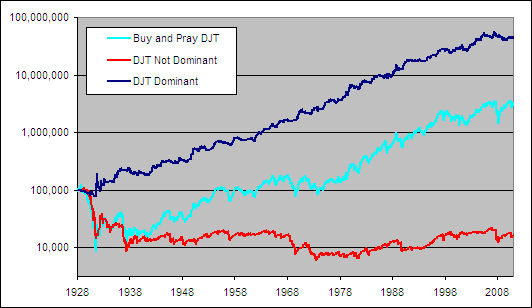
TransDow Performance

The dark blue line on the chart above is the result of nothing more that EOW data, a ratio, a simple moving average and a stop loss! Only exposed to the market 45% of the time it achieved an annualized return during exposure of 17.62% compared to the Buy and Pray annualized return from the DOW and DJT of just 4.55% and 4.24% respectively.

Note, research shows that only 17% of mutual funds beat the market and only 5% beat them by more than 1% per year. In fact the average actively managed stock mutual fund returns approximately 2% less per year to its shareholders than the stock market in general.

The TransDow could hardly be described as a complicated system. All the trading rules can be explained to a child in about 150 words. Yet despite its simplicity it succeeds in doing something that the MBAs running America’s Mutual Funds have failed to do; it outperforms the market and it had done so in a big way over a VERY long time.

So what are the Transports doing during the times when the Smart Money is seeking safety and the Dow is dominant?

During the test period of 83 years DJT advanced 3,033%. However if you only had your money in DJT during the 50% of the time that the Dow was dominant over the Transports then you would have lost 84% (see red line on chart above). This is very compelling evidence to back up the theory that when the more economically sensitive Transports are dominant the vast majority of market gains occur and vice versa.

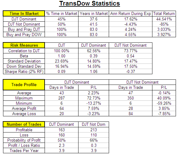
TransDow Stats

The Problem

So we have demonstrated this system working consistently over an 83 year period. That is nothing insignificant and I challenge you to provide an example of another system that can do the same over such a time frame. Despite this, we are not happy and do not view this model as being robust enough. The reason is simple, care to guess as to what it is? Leave your thoughts in the comments section below.

Double Vs Triple Exponential Moving Average

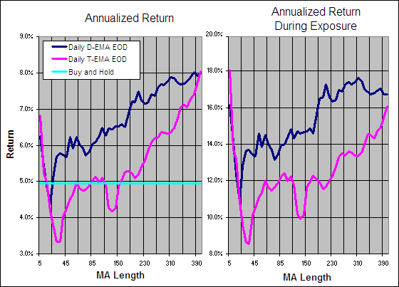
In this round of testing we are looking at the Double Exponential (D-EMA) and Triple Exponential Moving Averages (T-EMA). We have already tested the D-EMA and found that it wasn’t as effective as the EMA but wanted to test it over longer periods and compare it to the T-EMA.

In conducting these tests we measured the performance of each indicator going Long and Short, using Daily and Weekly data, taking End Of Day (EOD) and End Of Week (EOW) signals with smoothing periods varying from from 5 – 400 days or 80 weeks.~ These tests were carried out over a total of 300 years of data across 16 different global indexes (details here).

Note – Due to the huge lead in period required for the T-EMA, 240 weeks of data was ‘left in’ on each market. As a result the average buy and hold annualized return for the test markets was 4.94%. In our previous tests we only ‘left in’ 104 weeks and the subsequent buy and hold annualized return for the test markets was 6.32%. For this reason the results for these tests are not directly comparable to our other tests results. This is also why the returns for the D-EMA displayed below are lower than those previously published.

Triple and Double Exponential MA Annualized Return

Above are the return statistics when going long using daily, end of day signals. As you can see the Triple EMA under performs the Double EMA by a significant margin. Due to the fact that we have already established that the D-EMA is not worthy of use in a trading system the same can be said for the T-EMA and therefore there is no point in displaying any more statistics for these indicators. See also – Simple Vs Exponential Moving Averages

~ An entry signal to go long (or exit signal to cover a short) for each average tested was generated with a close above that average and an exit signal (or entry signal to go short) was generated on each close below that moving average. No interest was earned while in cash and no allowance has been made for transaction costs or slippage. Trades were tested using End Of Day (EOD) and End Of Week (EOW) signals for Daily data and EOW signals only for Weekly data. Eg. Daily data with an EOW signal would require the Week to finish above a Daily Moving Average to open a long or close a short and vice versa.

Double (D-EMA) and Triple Exponential Moving Average (T-EMA)

The Double and Triple Exponential Moving Average were created by Patrick Mulloy and first published in the February 1994 issue of Technical Analysis of Stocks & Commodities magazine – Smoothing Data With Less Lag. Mulloy stated in his article:

“Moving averages have a detrimental lag time that increases as the moving average length increases. The solution is a modified version of exponential smoothing with less lag time.”

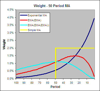
Like an EMA, the D-EMA and T-EMA apply more weight to the most recent data in an attempt to smooth out noise while still remaining highly reactive to changes in the data. This is not achieved by simply double and triple smoothing as one may assume. To do so results in weighting that resembles a backwards log-normal distribution, rather like a Triangular Moving Average but smooth and shifted forward. Below you can see how the weighting is allocated by a single, double and triple smoothed exponential moving average compared to a standard EMA and SMA:

Double and Tripple Smoothed EMA Weighting .

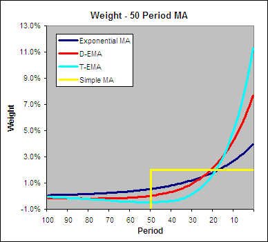
As you can see by double and triple smoothing an EMA the weighting no longer focuses on the latest data. The actual Double and Triple Exponential Moving Average applies the weighing very heavily to the most recent data as illustrated in the chart below:

Double and Tripple EMA Weight

How To Calculate a Double Exponential Moving Average and T-EMA

Double Exponential MA Formula:

D-EMA = 2*EMA – EMA(EMA)

Triple Exponential MA Formula:

T-EMA = (3*EMA – 3*EMA(EMA)) + EMA(EMA(EMA))

Where:

EMA = EMA(1) + α * (Close – EMA(1))

α = 2 / (N + 1)

N = The smoothing period.

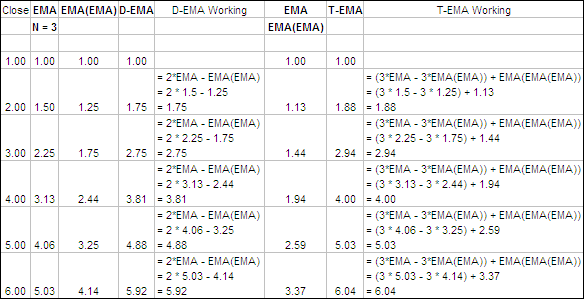
Here is an example of a 3 period Double Exponential Moving Average and Triple EMA:

Double and Triple Exponential Moving Average Formula .

Triple Exponential Moving Average and D-EMA Excel File

We have built a spreadsheet to calculate the D-EMA and T-EMA and have made it available for free download. Find the file at the following link near the bottom of the page under Downloads – Technical Indicators: Double (D-EMA) and Triple Exponential Moving Average (T-EMA).

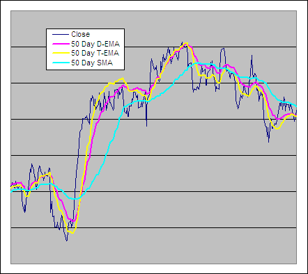
Double EMA, Triple EMA and a Simple Moving Average

Double and Tripple EMA Vs a Simple MA .

Double and Triple Exponential Moving Average Test Results

We ran them through tests through over 300 years of data across 16 different global markets. Here are the results:

Double Exponential Moving average Vs Simple and Exponential Moving average

Double Vs Triple Exponential Moving Average

More in this series:

We have conducted and continue to conduct extensive tests on a variety of technical indicators. See how they perform and which reveal themselves as the best in the Technical Indicator Fight for Supremacy.

Mixed Moving Averages – Test Results

In this round of testing we will be looking at a mix of different smoothing methods and averages: The Moving Linear Regression or Time Series Forecast (TSF) and The Linear Regression Indicator (LRI) which aren’t actually moving averages but can be used in the same way. Plus Wilder’s Smoothing AKA Smoothed MA (WS-MA) and the Triangular Simple MA (TriS-MA). The aim is to identify if any of these indicators are worth using as a trading tool.

We tested each indicator going Long and Short, using Daily and Weekly data, taking End Of Day (EOD) and End Of Week (EOW) signals with smoothing periods varying from from 5 – 300 days or 60 weeks.~ These tests were carried out over a total of 300 years of data across 16 different global indexes (details here).

Annualized Return Mixed Moving Averages

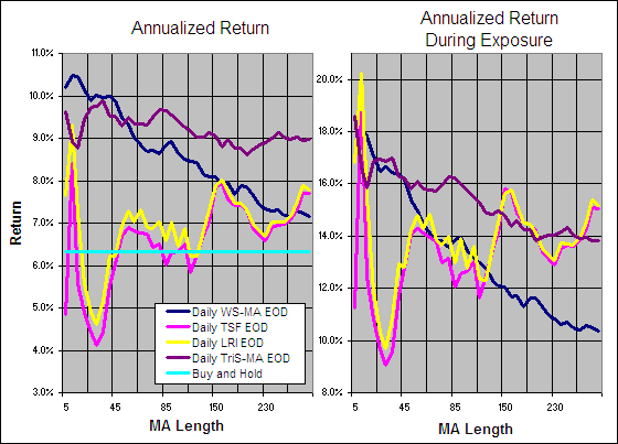
Above you can see the annualized return statistics for each indicator. The first thing that you will notice is that the LRI and TSF produce very similar results and neither of them are very good. So for providing buy signals in this fashion the Time Series Forecast and The Linear Regression Indicator are knocked out cold in the first round.

The returns generated by the TriS-MA are reasonable but they are not good enough to out perform the EMA’s results so the Triangular Simple Moving Average is also knocked out of contention. (Note – It didn’t dawn on us that the TriS-MA is almost identical to the Triangular Weighted Moving Average until after we had already tested it).

Wilder’s Smoothing produced some good returns when the smoothing period was less than 45 days but the performance dropped gradually to almost 7% as the length was extended. The EMA exhibited similar behavior but bottomed out around 8% so while Wilder’s Smoothing is effective in this application, the Exponential Moving Average is still King.
.

Best Average of the Group – Long

We performed a total of 948 tests in this round; half of them on the long side and half on the short. Rather than simply selecting the indicator with the greatest returns over the test period we identified the best for going long using the following criteria:

Annualized Return > 9%
Average Trade Duration > 29 Days
Annualized Return During Exposure > 15%
Annualized Return on Nikkei 225 > 3%

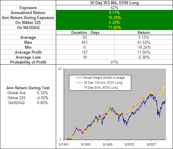
14/357 Averages made the final cut (see spreadsheet) but we selected the 30 Day Wilder’s Smoothing with End of Week Signals as the ultimate winner:
.

30 Day WS-MA, EWO Long .

Above you can see how the 30 Day WS-MA, EOW Long performed during the test period compared to the 75 Day EMA, EOW Long which was selected as the most effective Exponential Moving Average in a previous test. The WS-MA with this particular smoothing period produced almost identical results to the EMA but didn’t offer any benefits.

Upon further testing we found that despite very different calculation the WS-MA and the EMA are actually the same indicator. Simply double the WS-MA period and subtract one to find the equivalent EMA. For instance a 38 period WS-MA is identical to a 75 period EMA.

– The average annualized return of the 16 markets during the testing period was 6.32%. The data used for these tests is included in the results spreadsheet and more details about our methodology can be found here.

Exponential Moving Average (EMA)

The Exponential Moving Average (EMA) is a very popular method for smoothing data in an attempt to eliminate noise and our tests show that it is also highly effective. Unlike the Simple Moving Average (SMA) that applies equal weight to all data, the EMA applies more weight to the recent data so that it reacts faster to sudden changes.

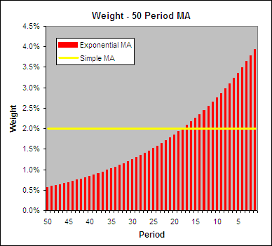
You can see see why it is called an Exponential Moving Average when you look at how the weighting is applied; it is in the shape of an exponential curve. Because of this the weighting never reaches zero and the influence of early data always remains (although it has little effect outside of the specified smoothing period). This is more clearly illustrated by the chart below which shows the weighting for a 50 period EMA and a SMA:

Weighting - Exponential Moving Average and a SMA .

Although we call it a 50 period EMA, those 50 periods only actually account for 86% of the weighting. A further 12% is applied over the preceding 50 periods leaving the last 2% to be spread amongst all the prior data. Here is a great article from MarketSci on this topic: Visual Depiction of SMA vs EMA Weighting

How To Calculate an Exponential Moving Average

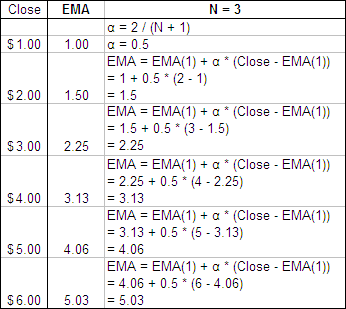
Calculating an Exponential Moving Average actually requires less processing power than a Simple Moving Average because it only refers to the current period and the previous EMA value. While it does not become active until the Nth period the EMA starts with the first close price and after that is calculated according to the following formula:

EMA = EMA(1) + α * (Close – EMA(1))

Where:

α = 2 / (N + 1)

N = The smoothing period.

Here is an example of a 3 period Exponential Moving Average:

How to Calculate an Exponential Moving Average

If you have two data sets and you wish to find out the EMA smoothing period, the following formula will reveal it:

N = (2-( (MA-MA[1]) / (Close-MA[1]) ) ) / ( (MA-MA[1]) / (Close-MA[1]) )

Exponential Moving Average Excel File

The EMA is so simple to calculate that it is unlikely that you would need a version in Excel but we have put together one for those of you that are lazy :). It is free and contains the ‘basic’ version you can see above and one that will automatically adjust to the length you specify. Find it at the following link near the bottom of the page under Downloads – Technical Indicators: Exponential Moving Average (EMA).

Exponential Moving Average and a Simple Moving Average

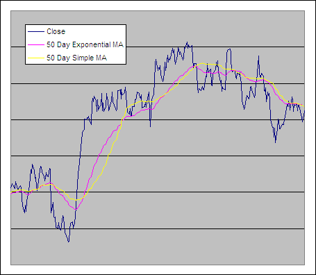
Exponential Moving Average vs Simple MA .

Test Results

If you haven’t already then check out the EMA test results. We tested it against the SMA and D-EMA through 300 years of data across 16 global markets to reveal which is the best and the characteristics they exhibit as their smoothing period is changed. See the results; Moving Averages – Simple vs Exponential

Simple Moving Average (SMA)

The Simple Moving Average or SMA is probably the most commonly used technical indicator of all. It can be calculated by taking the average of a data series (usually the close price) over a set number of periods. As each period progresses the last value is dropped out of the calculation and the latest one takes its place; hence the ‘Moving’ characteristic.

Financial data is notorious for being full of noise. Smoothing methods like averages help to filter out some of that noise so that a clearer picture of what is really going on can be revealed. Test results show however the Simple Moving Average is certainly not the most effective smoothing method available. Why then do we use the SMA in the weekly ETF HQ Report?

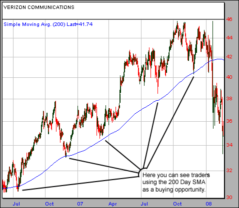
Some Simple Moving Averages such as the 50, 100 and 200 day SMA are so widely followed that they regularly become important support and resistance levels. There is no reason why this should happen other than the fact that they have become a self fulfilling prophecy. If enough people think that a level is important then it becomes important:

200 Day Simple Moving Average as Support .

Above is an example the 200 day SMA acting as support and being seen as a buying opportunity for over a year. With so many points of inflection on this average the eventual break was viewed by traders as a significant technical failure and a flood of selling ensued.

For those of you who use Excel in your trading I have built a spreadsheet for you that contains a simple moving average. You are probably wondering why you would want to download such a simple indicator but this one is useful because it will automatically adjust to the length that you specify. We find this a useful feature and hopefully you will as well. Get the file at the following link near the bottom of the page under Downloads – Technical Indicators: Simple Moving Average (SMA). Please let us know if you find it useful.

Moving Average Test Results

Have you ever wondered which is better; a simple or exponential moving average? Well we tested both along with a double exponential moving average through 300 years of data across 16 global markets to reveal the answer. Here are the results – Simple vs. Exponential Moving Average