Standard Deviation Ratio Variable Moving Ave (SDR-VMA) – Test Results

The Variable Moving Average (VMA) dynamically adjusts its own smoothing period to the changing market conditions based on a Volatility Index (VI). While any VI can be used, in this article we will look at how the VMA performs using a Standard Deviation Ratio (SDR). This is the VI that Tushar S. Chande first suggested be used when he presented what he called a Volatility Index Dynamic Average (VIDYA) in the March 1992 edition of Technical Analysis of Stocks & Commodities – Adapting Moving Averages To Market Volatility.

The SDR-VMA requires three user selected inputs: A Short Standard Deviation (SD1), a Longer Standard Deviation (SD2) and a VMA period. We tested trades going Long and Short, using Daily data, taking End Of Day (EOD) and End Of Week (EOW) signals~ analyzing all combinations of:

SD1 = 10, 20, 40, 80, 126

SD2 = 20, 40, 80, 126, 252

VMA = 5, 10, 15, 20, 25, 30, 35, 40, 45, 50

The SD lengths were selected due to the fact that they correspond with the approximate number of trading days in standard calendar periods: 10 days = 2 weeks, 20 days = 1 month, 40 days = 2 months, 80 days = ⅓ year, 126 days = ½ year and there are 252 trading days in an average year.

The VMA periods were selected after preliminary tests showed that when combined with the different SDR combinations, these settings resulted in a median smoothing period between 6 and 280 days; a range that should capture the best results based on what we know from previous research into moving averages.

A total of 390 different averages were tested and each one was run through 300 years of data across 16 different global indexes (details here).

Download A FREE Spreadsheet With Raw Data For

All 390 SDR-VMA Long and Short Test Results

SDR Variable Moving Average Test Results, Daily EOD, Long:

The data collected from our tests has been split by SD1 length with return plotted on the “y” axis, the VMA constant on the “x” axis and a separate series displayed for each SD2 length.

VIDYA Annualized Return .

First up it must be noted that every single SDR-VMA Long using EOD signals on Daily data outperformed the average buy and hold annualized return of 6.32%^ during the test period (before allowing for transaction costs and slippage). This is a vote of confidence for the concept especially seeing as each average was typically sitting in cash 37% of the time.

Perhaps the most interesting information from the data however is the fact that the best performer from each set had a SD2 that was twice the length of SD1. This formula of SD2 = 2*SD1 should therefore be used whenever utilizing the Standard Deviation Ratio.

The Best SDR-VMA Parameters

The best performing average was found where SD1 = 126, SD2 = 252 and the VMA constant = 5. In the FRAMA tests we also saw that the periods of 126 (half a year) and 252 (a full trading year) produced the best results so this appears to be a reoccurring theme:

126, 252 Day SDR-VMA, EOD 5, Long .

I have included on the above chart the performance of the 126 Day FRAMA, EOD 4, 300 Long becuase so far this has been the best performing Moving Average and as you can see the SDR-VMA under performs. To make matters worse it has an typical trade duration of just 9 days compared to the FRAMA’s 14, and underperformed the buy and hold returns of both the Nikkei 225 and the NASDAQ. Therefore we can conclude that the SDR-VMA, despite being effective is not as good as the FRAMA.

A look at the Smoothing Period:

126, 252 Day SDR-VMA, EOD 5 - Smoothing Period Distribution .

By looking at the smoothing distribution you can see why the SDR-VMA is so much faster than the FRAMA. While the FRAMA has a range of 293 days and a median of 21, the SDR-VMA has a range of just 37 days and a median of 8.

126, 252 Day SDR-VMA, 5 – Alpha Comparison

To get an idea of the readings that created these results we charted a section of the alpha for the 126, 252 Day SDR-VMA, 5 and compared it to the best performing FRAMA to see if there were any similarities that would reveal what makes a good volatility index:

126, 252 Day SDR-VMA, 5 - Alpha Comparison .

The alpha patterns are similar for both the 126 Day FRAMA 4, 300 and the 126, 252 Day SDR-VMA 5 but the readings are still very different. The SDR-VMA’s indicator is nearly always higher than the FRAMA’s which is why the resulting VMA is much faster.

It is desirable to see however that the SDR-VMA’s alpha is so clean and noise free in its movements. This leads me to believe that the 126, 252 SDR would be a good VI if it were adjusted to produce a slower average. Also due to the lack of noise from the SDR it may offer value in other applications such a way of ranking a universe of stocks by their trend strength, but that is the topic of another set of tests.

For more in this series see – Technical Indicator Fight for Supremacy

~ An entry signal to go long (or exit signal to cover a short) for each average tested was generated with a close above that average and an exit signal (or entry signal to go short) was generated on each close below that moving average. No interest was earned while in cash and no allowance has been made for transaction costs or slippage. Trades were tested using End Of Day (EOD) and End Of Week (EOW) signals on Daily data. Eg. Daily data with an EOW signal would require the Week to finish above a Daily Moving Average to open a long or close a short while Daily data with EOD signals would require the Daily price to close above a Daily Moving Average to open a long or close a short and vice versa.
^ This was the average annualized return of the 16 markets during the testing period. The data used for these tests is included in the results spreadsheet and more details about our methodology can be found here.

Double Vs Triple Exponential Moving Average

In this round of testing we are looking at the Double Exponential (D-EMA) and Triple Exponential Moving Averages (T-EMA). We have already tested the D-EMA and found that it wasn’t as effective as the EMA but wanted to test it over longer periods and compare it to the T-EMA.

In conducting these tests we measured the performance of each indicator going Long and Short, using Daily and Weekly data, taking End Of Day (EOD) and End Of Week (EOW) signals with smoothing periods varying from from 5 – 400 days or 80 weeks.~ These tests were carried out over a total of 300 years of data across 16 different global indexes (details here).

Note – Due to the huge lead in period required for the T-EMA, 240 weeks of data was ‘left in’ on each market. As a result the average buy and hold annualized return for the test markets was 4.94%. In our previous tests we only ‘left in’ 104 weeks and the subsequent buy and hold annualized return for the test markets was 6.32%. For this reason the results for these tests are not directly comparable to our other tests results. This is also why the returns for the D-EMA displayed below are lower than those previously published.

Triple and Double Exponential MA Annualized Return

Above are the return statistics when going long using daily, end of day signals. As you can see the Triple EMA under performs the Double EMA by a significant margin. Due to the fact that we have already established that the D-EMA is not worthy of use in a trading system the same can be said for the T-EMA and therefore there is no point in displaying any more statistics for these indicators. See also – Simple Vs Exponential Moving Averages

~ An entry signal to go long (or exit signal to cover a short) for each average tested was generated with a close above that average and an exit signal (or entry signal to go short) was generated on each close below that moving average. No interest was earned while in cash and no allowance has been made for transaction costs or slippage. Trades were tested using End Of Day (EOD) and End Of Week (EOW) signals for Daily data and EOW signals only for Weekly data. Eg. Daily data with an EOW signal would require the Week to finish above a Daily Moving Average to open a long or close a short and vice versa.

Mixed Moving Averages – Test Results

In this round of testing we will be looking at a mix of different smoothing methods and averages: The Moving Linear Regression or Time Series Forecast (TSF) and The Linear Regression Indicator (LRI) which aren’t actually moving averages but can be used in the same way. Plus Wilder’s Smoothing AKA Smoothed MA (WS-MA) and the Triangular Simple MA (TriS-MA). The aim is to identify if any of these indicators are worth using as a trading tool.

We tested each indicator going Long and Short, using Daily and Weekly data, taking End Of Day (EOD) and End Of Week (EOW) signals with smoothing periods varying from from 5 – 300 days or 60 weeks.~ These tests were carried out over a total of 300 years of data across 16 different global indexes (details here).

Annualized Return Mixed Moving Averages

Above you can see the annualized return statistics for each indicator. The first thing that you will notice is that the LRI and TSF produce very similar results and neither of them are very good. So for providing buy signals in this fashion the Time Series Forecast and The Linear Regression Indicator are knocked out cold in the first round.

The returns generated by the TriS-MA are reasonable but they are not good enough to out perform the EMA’s results so the Triangular Simple Moving Average is also knocked out of contention. (Note – It didn’t dawn on us that the TriS-MA is almost identical to the Triangular Weighted Moving Average until after we had already tested it).

Wilder’s Smoothing produced some good returns when the smoothing period was less than 45 days but the performance dropped gradually to almost 7% as the length was extended. The EMA exhibited similar behavior but bottomed out around 8% so while Wilder’s Smoothing is effective in this application, the Exponential Moving Average is still King.
.

Best Average of the Group – Long

We performed a total of 948 tests in this round; half of them on the long side and half on the short. Rather than simply selecting the indicator with the greatest returns over the test period we identified the best for going long using the following criteria:

Annualized Return > 9%
Average Trade Duration > 29 Days
Annualized Return During Exposure > 15%
Annualized Return on Nikkei 225 > 3%

14/357 Averages made the final cut (see spreadsheet) but we selected the 30 Day Wilder’s Smoothing with End of Week Signals as the ultimate winner:
.

30 Day WS-MA, EWO Long .

Above you can see how the 30 Day WS-MA, EOW Long performed during the test period compared to the 75 Day EMA, EOW Long which was selected as the most effective Exponential Moving Average in a previous test. The WS-MA with this particular smoothing period produced almost identical results to the EMA but didn’t offer any benefits.

Upon further testing we found that despite very different calculation the WS-MA and the EMA are actually the same indicator. Simply double the WS-MA period and subtract one to find the equivalent EMA. For instance a 38 period WS-MA is identical to a 75 period EMA.

– The average annualized return of the 16 markets during the testing period was 6.32%. The data used for these tests is included in the results spreadsheet and more details about our methodology can be found here.

Weighted Moving Averages Put To The Test

A Weighted Moving Average smooths data by setting a separate but specific weighting for each data set over the length of its smoothing period. In this round of testing we will look at the standard Weighted Moving Average (W-MA), the Triangular Weighted Moving Average (TriW-MA) and the Sine Weighted Moving Average (SW-MA) in order to reveal which is the best and if any of them are worth including in your trading tool box.

To evaluate these averages we tested Long and Short trades using Daily and Weekly data, taking End Of Day (EOD) and End Of Week (EOW) signals with Moving Average lengths varying from from 5 – 300 days or 60 weeks.~ These tests were carried out over a total of 300 years of data across 16 different global indexes (details here).

Weighted Moving Average – Test Conclusion

Weighted Moving Average - Long and Short Annualized Return

Above you can see how the annualized return changes with the length of each Daily, EOD Moving Average for the Long and the Short side of the market. The relative performance of each MA was similar when going Long or Short but the returns on the Short side were much lower.

There is little difference in performance between the TriW-MA and the SW-MA while the W-MA was clearly superior. The W-MA performed particularly well with a setting of 35 days or 110 days, peaking with a annualized return of over 10% on these settings. As the smoothing period is extended beyond 110 days the returns gradually diminished.

Return to Top

Weighted Moving Average - Long and Short Annualized Return During Exposure

Above you can see the performance of each average during the time that it was exposed to the market. Across the board the efficiency of each average decreased as the length of each average is was increased. The W-MA again proved the most effective.

Return to Top

Best Weighted Moving Average – Long

We tested 357 averages on the Long side but rather than simply selecting the one with the greatest returns over the test period we looked for the following criteria:

Annualized Return > 9%
Average Trade Duration > 29 Days
Annualized Return During Exposure > 15%
Annualized Return on Nikkei 225 > 3%
Annualized Return on NASDAQ > 12.5%

8/357 Averages made the final cut (see spreadsheet) but we selected the 90 Day Weighted Moving Average with End of Week Signals as the ultimate winner:
.

90 Day W-MA, EOW Long

.
Above you can see how the 90 Day W-MA, EOW Long performed during the test period compared to the 75 Day EMA, EOW Long which was selected as the most effective Exponential Moving Average in a previous test. The Weighted MA produced very similar results to the EMA but didn’t offer any benefits.

Return to Top

Weighted Moving Average – Test Conclusion

The Triangular and Sine Weighted Moving Averages proved to be inferior to the W-MA while the standard Weighted Moving Average did produce reasonable returns. Those returns however, were similar (if slightly inferior) to those of an Exponential Moving Average while not offering any notable benefits. Therefore it can be concluded that none of the Weighted Moving Averages we tested are worth perusing further.

Return to Top

FRAMA – Is It Effective?

The Fractal Adaptive Moving Average aka FRAMA is a particularly clever indicator. It uses the Fractal Dimension of stock prices to dynamically adjust its smoothing period. In this post we will reveal how the FRAMA performs and if it is worthy of being included in your trading arsenal.

To fully understand how the FRAMA works please read this post before continuing. You can also download a FREE spreadsheet containing a working FRAMA that will automatically adjust to the settings you specify. Find it at the following link near the bottom of the page under Downloads – Technical Indicators: Fractal Adaptive Moving Average (FRAMA). Please leave a comment and share this post if you find it useful.

The ‘Modified FRAMA’ that we tested consists of more than one variable. So before we can put it up against other Adaptive Moving Averages to compare their performance, we must first understand how the FRAMA behaves as its parameters are changed. From this information we can identify the best settings and use those settings when performing the comparison with other Moving Average Types.

Each FRAMA requires a setting be specified for the Fast Moving Average (FC), Slow Moving Average (SC) and the FRAMA period itself. We tested trades going Long and Short, using Daily and Weekly data, taking End Of Day (EOD) and End Of Week (EOW) signals~ analyzing all combinations of:

FC = 1, 4, 10, 20, 40, 60

SC = 100, 150, 200, 250, 300

FRAMA = 10, 20, 40, 80, 126, 252

Part of the FRAMA calculation involves finding the slope of prices for the first half, second half and the entire length of the FRAMA period. For this reason the FRAMA periods we tested were selected due to being even numbers and the fact that they correspond with the approximate number of trading days in standard calendar periods: 10 days = 2 weeks, 20 days = 1 month, 40 days = 2 months, 80 days = ⅓ year, 126 days = ½ year and there are 252 trading days in an average year. A total of 920 different averages were tested and each one was run through 300 years of data across 16 different global indexes (details here).

Download A FREE Spreadsheet With Raw Data For

All 920 FRAMA Long and Short Test Results

FRAMA – Test Results:

Daily vs Weekly Data – EOD vs EOW Signals
Annualized Return
Annualized Return During Exposure
Time In The Market
Trade Duration
Probability Of Profit

Best FRAMA Parameters

Fast FRAMA Smoothing Distribution

A Slower FRAMA

Slow FRAMA Smoothing Distribution

FRAMA Testing – Conclusion

Daily vs Weekly Data – EOD vs EOW Signals

In our original MA test; Moving Averages – Simple vs. Exponential we revealed that once an EMA length was above 45 days, by using EOW signals instead of EOD signals you didn’t sacrifice returns but did benefit from a 50% jump in the probability of profit and double the average trade duration. To see if this was also the case with the FRAMA we compared the best returns produced by each signal type:

FRAMA - Best Returns by Signal Type

As you can see, for the FRAMA, Daily data with EOD signals produced by far the most profitable results and we will therefore focus on this data initially. It is presented below on charts split by FRAMA period with the test results on the “y” axis, the Fast MA (FC) on the “x” axis and a separate series displayed for each Slow MA (SC).

Return to Top

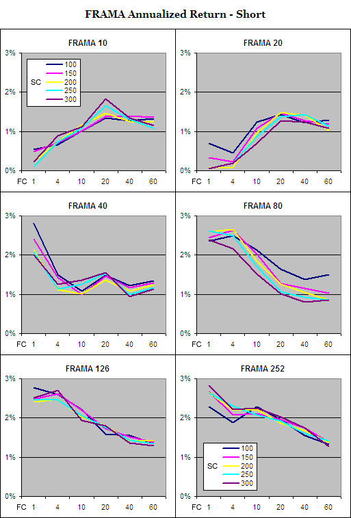
FRAMA Annualized Return – Day EOD Long

FRAMA - Annualized Return, Long

The first impressive thing about the results above is that every single Daily EOD Long average tested outperformed the buy and hold annualized return of 6.32%^ during the test period (before allowing for transaction costs and slippage). This is a strong vote of confidence for the FRAMA as an indicator.

You will also notice that the data series on each chart are all bunched together revealing that similar results are achieved despite the “SC” period ranging from 100 to 300 days. Changing the other parameters however makes a big difference and returns increase significantly once the FRAMA period is above 80 days. This indicates that the Fractal Dimension is not as useful if measured over short periods.

When the FRAMA period is short, returns increase as the “FC” period is extended. This is due to the Fractal Dimension being very volatile if measured over short periods and a longer “FC” dampening that volatility. Once the FRAMA period is 40 days or more the Fractal Dimension becomes less volatile and as a result, increasing the “FC” then causes returns to decline.

Overall the best annualized returns on the Long side of the market came from a FRAMA period of 126 days which is equivalent to about six months in the market, while a “FC” of just 1 to 4 days proved to be most effective. Assessing the results from the Short side of the market comes to the same conclusion although the returns were far lower: FRAMA Annualized Return – Short.

Return to Top

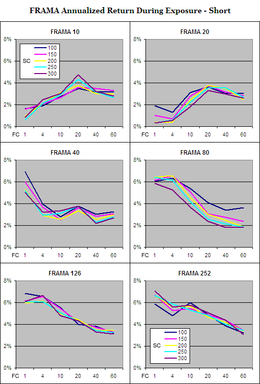
FRAMA Annualized Return During Exposure – Day EOD Long

FRAMA, Annualized Return During Exposure - Long .

The above charts show how productive each different Daily FRAMA EOD Long was while exposed to the market. Clearly the shorter FRAMA periods are far less productive and anything below 40 days is not worth bothering with. The 126 day FRAMA again produced the best returns with the optimal “FC” being 1 – 4 days. Returns for going short followed a similar pattern but as you would expect were far lower; FRAMA Annualized Return During Exposure – Short.

Moving forward we will focus in on the characteristics of the 126 Day FRAMA because it consistently produced superior returns.

Return to Top

FRAMA, EOD – Time in Market

FRAMA, Market Exposure - Long and Short .

Because the 16 markets used advanced at an average annualized rate of 6.32%^ during the test period it doesn’t come as a surprise that the majority of the market exposure was to the long side. By extending the “FC” it further increased the time exposed to the long side and reduced exposure on the short side. If the test period had consisted of a prolonged bear market the exposure results would probably be reversed.

Return to Top

FRAMA, EOD – Trade Duration

126 Day FRAMA, Average Trade Duration - Long & Short

By increasing the “FC” period it also extends the average trade duration. Changing the “SC” makes little difference but as the “SC” is raised from 100 to 300 days the average trade duration does increase ever so slightly.

Return to Top

FRAMA, EOD – Probability of Profit

126 Day FRAMA, Probability of Profit - Long & Short

As you would expect, the probability of profit is higher on the long side which again is mostly a function of the global markets rising during the test period. However the key information revealed by the charts above is that the probability of profit decreases significantly as the “FC” is extended. This is another indication that the optimal FRAMA requires a short “FC” period.

Return to Top

The Best Daily EOD FRAMA Parameters

Our tests clearly show that a FRAMA period of 126 days will produce near optimal results. While for the “SC” we have shown that any setting between 100 and 300 days will produce a similar outcome. The “FC” period on the other hand must be short; 4 days or less. John Ehlers’ original FRAMA had a “FC” of 1 and a “SC” of 198; this will produce fantastic results without the need for any modification.

Because we prefer to trade as infrequently as possible we have selected a “FC” of 4 and a “SC” of 300 as the best parameters because these settings results in a longer average trade duration while still producing great returns on both the Long and Short side of the market:

FRAMA, EOD – Long

126 Day FRAMA, EOD 4, 300 Long

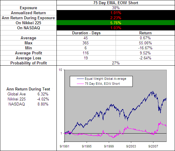
Above you can see how the 126 Day FRAMA with a “FC” of 4 and a “SC” of 300 has performed since 1991 compared to an equally weighted global average of the tested markets. I have included the performance of the 75 Day EMA, EOW becuase it was the best performing exponential moving average from our original tests.

This clearly illustrates that the Fractal Adaptive Moving Average is superior to a standard Exponential Moving Average. The FRAMA is far more active however producing over 5 times as many trades and did suffer greater declines during the 2008 bear market.

FRAMA, EOD – Short

126 Day FRAMA, EOD 4, 300 Short

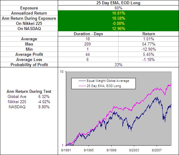
On the Short side of the market the FRAMA further proves its effectiveness. Without needing to change any parameters the 126 Day FRAMA, EOD 4, 300 remains a top performer. When we ran our original tests on the EMA we found a faster average worked best for going short and that the 25 Day EMA was particularly effective. But as you can see on the chart above the FRAMA outperforms again.

What is particularly note worthy is that the annualized return during the 27% of the time that this FRAMA was short the market was 6.64% which is greater than the global average annualized return of 6.32%.

See the results for the 126 Day FRAMA, EOD 4, 300
Long and Short on each of the 16 markets tested.

Return to Top

126 Day FRAMA, EOD 4, 300 – Smoothing Period Distribution

With a standard EMA the smoothing period is constant; if you have a 75 day EMA then the smoothing period is 75 days no matter what. The FRAMA on the other hand is adaptive so the smoothing period is constantly changing. But how is the smoothing distributed? Does it follow a bell curve between the “FC” and “SC”, is it random or is it localized around a few values. To reveal the answer we charted the percentage that each smoothing period occurred across the 300 years of test data:

126 Day FRAMA, EOD 4, 300 - Smoothing Period Distribution .

The chart above came as quite a surprise. It reveals that despite a “FC” to “SC” range of 4 to 300 days, 72% of the smoothing was within a 4 to 50 day range and the majority of it was only 5 to 8 days. This explains why changing the “SC” has little impact and why changing the “FC” makes all the difference. It also explains why the FRAMA does not perform well when using EOW signals, as an EMA must be over 45 days in duration before EOW signals can be used without sacrificing returns.

Return to Top

A Slower FRAMA

.
We have identified that the FRAMA is a very effective indicator but the best parameters (126 Day FRAMA, EOD 4, 300 Long) result in a very quick average that in your tests had an typical trade duration of just 14 days. We also know that the 75 Day EMA, EOW Long is an effective yet slower moving average and in our tests had a typical trade duration of 74 days.

A good slow moving average can be a useful component in any trading system because it can be used to confirm the signals from other more active indicators. So we looked through the FRAMA test results again in search a less active average that is a better alternative to the 75 Day EMA and this is what we found:

252 Day FRAMA, EOW 40, 250 Long .

The 252 Day FRAMA, EOW 40, 250 Long produces some impressive results and does out perform the 75 Day EMA, EOW Long by a fraction. However this fractional improvement is in almost every measure including the performance on the short side. The only draw back is a slight decrease in the average trade duration from 74 days to 63 when long. As a result the 252 Day FRAMA, EOW 40, 250 has knocked the 75 Day EMA, EOW out of the Technical Indicator Fight for Supremacy.

See the results for the 252 Day FRAMA, EOW 40, 250
Long and Short on each of the 16 markets tested.

Return to Top

252 Day FRAMA, EOW 40, 250 – Smoothing Period Distribution

252 Day FRAMA, EOW 40, 250 - Smoothing Period Distribution .

Return to Top

FRAMA Testing – Conclusion

The FRAMA is astoundingly effective as both a fast and a slow moving average and will outperform any SMA or EMA. We selected a modified FRAMA with a “FC” of 4, a “SC” of 300 and a “FRAMA” period of 126 as being the most effective fast FRAMA although the settings for a standard FRAMA will also produce excellent results. For a slower or longer term average the best results are likely to come from a “FC” of 40, a “SC” of 250 and a “FRAMA” period of 252.

Robert Colby in his book ‘The Encyclopedia of Technical Market Indicators’ concluded, “Although the adaptive moving average is an interesting newer idea with considerable intellectual appeal, our preliminary tests fail to show any real practical advantage to this more complex trend smoothing method.” Well Mr Colby, our research into the FRAMA is in direct contrast to your findings.

It will be interesting to see if any of the other Adaptive Moving Averages can produce better returns. We will post the results HERE as they become available.

Well done John Ehlers you have created another exceptional indicator!

More in this series:

We have conducted and continue to conduct extensive tests on a variety of technical indicators. See how they perform and which reveal themselves as the best in the Technical Indicator Fight for Supremacy.

Return to Top

~ An entry signal to go long (or exit signal to cover a short) for each average tested was generated with a close above that average and an exit signal (or entry signal to go short) was generated on each close below that moving average. No interest was earned while in cash and no allowance has been made for transaction costs or slippage. Trades were tested using End Of Day (EOD) and End Of Week (EOW) signals for Daily data and EOW signals for Weekly data. Eg. Daily data with an EOW signal would require the Week to finish above a Daily Moving Average to open a long or close a short while Daily data with EOD signals would require the Daily price to close above a Daily Moving Average to open a long or close a short and vice versa.
^ This was the average annualized return of the 16 markets during the testing period. The data used for these tests is included in the results spreadsheet and more details about our methodology can be found here.

ETF % Change Comparison

Each week in the ETF HQ report we look at a percentage comparison on the performance of six ETFs. This group we refer to as ‘The Influential ETFs’ because they are highly influential in dictating the markets true direction. The group is made up of four ‘Economically Sensitive‘ (SMH, QQQQ, IWM and IYT) and two ‘Economically Stable‘ funds (SPY and DIA).

Example:

ETF % Change Comparison

The ‘Economically Sensitive’ ETFs amplify market movements rather like a Richter Scale amplifies the movements of the earth in order to warn of coming earth quakes and eruptions. While the more ‘Economically Stable’ ETFs are important to get a gauge of relative performance; to provide a benchmark.

By comparing the performance of the economically sensitive and stable ETFs we can get an indication of the true market direction because the more sensitive areas are usually the first to initiate a trend change. For example if DIA and SPY sell off heavily while SMH and IWM sell of mildly or continue moving to new highs then this would be very positive and vice versa. By viewing the raw data in this ‘% Change Comparison’ we gain a useful additional perspective over just looking at the charts.

The Economically Sensitive:

SMH – Holds around 20 companies and is designed to provide exposure to the semiconductor industry. Today, in the information age this is arguably the most economically sensitive industry of all because it stands at the front of the business cycle. Semiconductors suffer periods of under and over supply that are uniquely linked to the speed of economic growth.

Because technology is advancing so quickly any inventory has a very short shelf life which results in painful loses for semiconductors before any other industry during a slowdown. This is why SMH is such a fantastic leading indicator for the direction and health of the broad market. Semiconductors play a similar role to that played by the rail roads during the industrial age and are useful as part of a modern Dow Theory.

QQQQ – Holds all the stocks in the NASDAQ 100 which is made up of the largest non-financial securities listed on the NASDAQ Stock Exchange. It is often referred to as the technology index becuase it is heavily weighted in the technology sector which is particularly economically sensitive. It is not possible for the economy to perform well without creating demand for services from the technology sector and technology stocks can’t perform well without their prosperity driving up demand for semiconductors. For this reason QQQQ tends to lead the broad market and SMH tends to lead QQQQ.

IWM – Holds about 90% of the securities in the Russell 2000 index in an attempt to track its performance. The Russell 2000 represents approximately 2000 of the smallest companies by market capitalization in the Russell 3000. While the Russell 3000 represents about 98% of the investable US market the Russell 2000 represents under 10%. These smaller companies have have the ability to grow much faster than their larger competitors when economic conditions are favorable but lack the stability of the large caps to weather storms as easily.

IYT – Tracks the Dow Jones Transportation Average and is comprised of companies involved in areas like air travel, trucking, railroads, air freight etc. Despite living in the information age, people and goods must still be moved in order for the wheels of industry to keep turning. If the Transports are performing well then it means that goods are being sold and this is a positive sign just as Dow observed in the his Dow Theory over 100 years ago.

The Economically Stable:

.
SPY – Emulates the S&P 500 which is designed to represent the 500 largest publicly traded US based companies by market capitalization. Due to the size of the companies that make up the S&P 500 it has a comparatively economically stable.

DIA – Tracks the Dow Jones Industrial Average which is made up of 30 Mega Cap US companies. These are ‘Blue Chip’ stocks that are considered some of the most stable and well established companies in the world making them about as economically stable as a public company can get.

Colors

.
The colors show the rank from 1-6 with 1 being the highest:

Moving Averages – Simple vs. Exponential

In this round of testing we put the Simple (SMA), Exponential (EMA) and Double Exponential (D-EMA) Moving Averages through their paces to identify which is the best and what characteristics can be expected as the length of each average is adjusted.

We tested Long and Short trades using Daily and Weekly data, taking End Of Day (EOD) and End Of Week (EOW) signals with Moving Average lengths varying from from 5 – 300 days or 60 weeks.~ These tests were carried out over a total of 300 years of data across 16 different global indexes (details here).

Simple vs. Exponential – Test Results:

Annualized Return
Annualized Return During Exposure
Trade Duration
Time In The Market
Biggest Loss
Probability Of Profit
Daily vs Weekly Data – EOD vs EOW Signals

Simple vs. Exponential Conclusion

Best Moving Average – Long
Best Moving Average – Short

Download A FREE Spreadsheet With All 948 Long and Short Test Results

Moving Average - Long and Short Annualized Return

Above you can see how the annualized return changes with the length of each Daily, EOD Moving Average for the Long and the Short side of the market. The relative performance of each MA is similar when going Long and Short but the returns on the Short side were much lower.

Both the SMA and EMAs spiked in return at 25 days and then returns steadily declined as the length of the averages increased, although the SMA did see some improved performance between 190 and 250 days. The D-EMA on the other hand is much faster and returns steadily improved as the Moving Average length increased from 20 through to 300 Days. (See Tests on the Triple Exponential Moving Average and D-EMA over longer periods – HERE.)

I was surprised to see that every single Daily, EOD Moving Average on the Long side outperformed the buy and hold annualized return of 6.32%^ during the test period (before allowing for transaction costs and slippage). On the Short side however, not a single average was able to beat the market during the test period. 5 – 75 Days appears to be the most effective zone, with the EMA proving to be superior to the SMA and D-EMA by annualized return.

Return to Top

Moving Average - Long and Short Annualized Return During Exposure

Above you can see the performance of each average during only the times that it actually had an open position. For the SMA and EMA the annualized return during exposure decreases as the length of the moving average is increased while the D-EMA exhibits the opposite behavior right up to the longest period we tested of 300 days. The 5 – 75 Day zone and the EMA also produce the best results by annualized return during exposure.

Return to Top

Moving Average - Trade Duration Long and Short

As would be expected, with an increase in the length of a moving average comes an increase in the duration of the trades that are generated. For all three classes of Moving Average tested, the duration of trades on the Short side was far less than those on the Long side. This is likely to be a function of two things – 1. The fact that the global markets gained an average of 6.32%^ annually during the test period, 2. Bull markets tend to be personified by slow and steady gains and bear markets tend to be faster and more violent.

From the above chart you also get an idea of just how much faster a D-EMA is. Notice how on the Long side, the average duration for a 300 Day, EOD D-EMA is similar to that of a 110 Day, EOD EMA or a 85 Day, EOD SMA.

Return to Top

Moving Average - Long and Short Time In The Market

Exposure to the market increases on the Long side and decreases on the Short side as the length of a moving average is increased. However the amount of exposure provided by the D-EMA levels off with each average above 140 Days long.

Return to Top

Moving Average - Long and Short Biggest Loss

There is no clear correlation between size of the largest single losing trade and the length of a moving average. However the D-EMA consistently suffers larger loses than the SMA and EMA on the Long side but after 90 Days tends to suffer smaller loses on the Short side.

Return to Top

Across the board, the probability of profit decreases as the length of an average increases but the D-EMA clearly identifies profitable trades more consistently than the SMA or EMA on both the Long and the Short side of the market.

Return to Top

Daily vs Weekly Data – EOD vs EOW Signals

Due to the superior performance of the EMA in the previous tests, lets take a closer look at how it behaves with Daily and Weekly data, taking EOD and EOW signals to see which combination is the most effective:

Exponential MA - Annualized Return Long

As you can see, there is a big difference between using EOD and EOW signals on the shorter averages but the results from Daily and Weekly data are very similar (Note – Each Daily average is compared to its Weekly equivalent eg. A 10 Day Average is compared to a 2 Week Average). Once the length of each average rises above 45 days the results for each data and signal combination become quite similar and above 100 days in length there is no tangible difference in return. The results are also similar on the Short side – EMA Annualized Return Short

Exponential MA - Probability of Profit and Trade Duration Long

By using EOW signals instead of EOD signals little is lost in the way of return but a large amount of noise is eliminated from the data. As a result, using EOW signals there is a jump in the probability of profit for each trade of almost 50% and the average trade duration is doubled! This clearly shows that taking EOW signals produces far more useful trades on averages above 45 days long. The results are similar on the Short side – EMA Probability of Profit and Trade Duration Short. The only real drawback of using EOW signals comes with a small jump in the size of the biggest loses incurred.

Return to Top

Simple vs Exponential – Conclusion

As a general rule we can conclude that the Exponential Moving Average is superior to both the Simple Moving Average and the Double Exponential Moving Average. It should be noted however that the D-EMA has some beneficial characteristics such as a higher probability of profit and greater returns during market exposure on the long side of the market.

It can also be said that there is very little difference between using Daily or Weekly data but using End Of Day signals will produce better results on shorter averages while End Of Week signals are just as effective on longer averages with the added benefit of a 50% jump in the probability of profit and double the trade duration.

Return to Top

Best Moving Average – Long

Rather than simply selecting the average with the greatest returns, in search of the very best we looked for:

Annualized Return > 9%
Average Trade Duration > 29 Days
Annualized Return During Exposure > 15%
Annualized Return on Nikkei 225 > 3%
Annualized Return on NASDAQ > 12.5%

.
Download A FREE Spreadsheet With All 948 Long and Short Test Results
.

9/474 Averages made the final cut (see spreadsheet) and any of them would make an effective trading tool but we selected the 75 Day Exponential Moving Average with End of Week Signals as the ultimate winner because it also produced good returns on the short side of the market:
.

Exponential MA - 75 Day, EOW Long
The 75 Day EMA, EOW Long has you exposed to the market 62% of the time and produces an average trade of 74 days in duration with a comparatively high 41% probability of profit. It also performed well on both the NASDAQ and ‘bear ravaged’ Nikkei 225. On the Short side it performed respectably as well; managing to endure the bullish periods by suffering only limited loses and making good returns when the market fell.

It will always be difficult for an indicator as basic as a Moving Average to successfully identify trades on the Short side during a period where the average market advanced 6.32%^ annually. However combined, the attributes of this particular Moving Average make it well suited for use in conjunction with other indicators as part of a complete trading system.

See the results for the 75 Day EMA, EOW
Long and Short on each of the 16 markets tested.

Return to Top

Best Moving Average – Short

The Short side of the market is very different to the long; cycles are faster and more volatile so the moving average most suited to a bear market is not necessarily the same as that most suited to a bull market. Of the 474 averages we tested on the Short side, in search of the very best we looked for:

Annualized Return > 0.5%
Average Trade Duration > 10 Days
Annualized Return During Exposure > 1.8%
Annualized Return on Nikkei 225 > 1.5%
Annualized Return on NASDAQ > 0.5%
Probability of Profit > 25%

6/474 Averages made the final cut (see spreadsheet) and any of them would make an effective trading tool but we selected the 25 Day Exponential Moving Average with End of Day Signals as the ultimate winner for Short trades because it produced the best returns out of the finalists:

25 Day EMA EOD - Short

The 25 Day EMA, EOD Short has you exposed to the market 40% of the time and produces an average trade of 12 days in duration with a comparatively high 25% probability of profit. By going with a much faster average on the Short side of the market, bearish profits are improved but this comes at the expense of more active trading. In the real market the more frequently you trade the greater your transaction costs, slippage and time required to execute the signals.

It is worth noting that this average performed O.K on the Nikkei 225 but didn’t produce outstanding results despite the Nikkei suffering a prolonged bear market during the test period. Surprisingly, the much longer 75 Day EMA, EOW Short (and several other averages above 45 days long) performed better than the 25 Day EMA, EOD Short on the Nikkei 225. This would suggest that a faster average has a better chance of making money on the Short side during a bull market but a slower average will produce better returns through a prolonged bear market. (Stats for bullish trades – 25 Day EMA, EOD Long)

See the results for the 25 Day EMA, EOD
Long and Short on each of the 16 markets tested.

More in this series:

Return to Top

~ An entry signal to go long (or exit signal to cover a short) for each average tested was generated with a close above that average and an exit signal (or entry signal to go short) was generated on each close below that moving average. No interest was earned while in cash and no allowance has been made for transaction costs or slippage. Trades were tested using End Of Day (EOD) and End Of Week (EOW) signals for both Daily and Weekly data. Eg. Daily data with an EOW signal would require the Week to finish above a Daily Moving Average to open a long or close a short while Weekly data with EOD signals would require the Daily price to close above a Weekly Moving Average to open a long or close a short and vice versa.
^ This was the average annualized return of the 16 markets during the testing period. The data used for these tests is included in the results spreadsheet and more details about our methodology can be found here.
* The ‘best averages’ highlighted on this table were selected by picking the top performers after averaging the returns of all four tests on each Moving Average length; Daily EOD, Daily EOW, Weekly EOD and Weekly EOW. Eg. The results for a 100 Day and the equivalent 20 Week Moving Average using both EOD and EOW signals have been averaged.

50 Day EMA, EOW Short

Technical Indicator – Fight for Supremacy

Which Technical Indicators are Best? There are a vast number of technical indicators out there but which ones are best? Are any of them suitable for use in a mechanical trading model? Do any of them actually provide value over a buy and hold approach? In my experience most of the publicly available technical indicators are of little, if any value. All of our best performing models are build on completely new ideas that deviate from conventional approaches to technical analysis almost entirely.

But questions remain: what length of moving average provides the best signals? Is it better to use a simple or exponential moving average? Quality answers to these questions are few and far between and often the process people use to establish such answers are majorly flawed.

Common Flaws in Testing Technical Indicators and Systems

Curve Fitting – Only Testing On One Stock or Index (usually the S&P 500) Even if a test period covers many years of data to only test one index will produce results that fit that curve. Also the US market has been one of the top performers over the last 100 years but will it be a top performer over the next 100? Japan has experienced a bear market over the last 20 years so vicious that it has seen the the Nikkei 225 down over 80% from its peak. To get an accurate idea of the effectiveness of an indicator it must be tested on several unrelated securities across the full spectrum of performance possibilities..
Testing A Range Of Individual Securities There are several misleading factors that come from testing a range of individual securities, the most troublesome one being the survivor-ship bias. If I was to test a random selection of stocks then one necessary criteria would be to select from a group of stocks that had been around long enough to provide adequate data for testing. But by selecting from stocks with enough data I would only be selecting randomly from stocks that had survived over that period and would be ignoring those that failed or had been de-listed. This is not how things work in the real world and would produce artificially inflated results..Another challenge with testing idividual securities is choosing the sellection criteria for which stocks to include. At which point should a cut off be made based on price, volume, market cap etc? Some stocks are going to have an excess or lack of volatility and there may be a large amount of noise in the data. This will make it difficult for even the best technical indicators to produce profitable signals and to limit losses.

.

A Less Flawed Method

There is no perfect way to test an indicator or system using historical data because past performance is no guarantee of future results. However the markets are driven by human emotion and crowd psychology. I believe that this behavior follows repeated patters and that effective historical testing can identify these patterns. In this way we can look to the past for an indication of the likely future.

In an attempt to be more effective at identifying patterns that are likely to repeat as opposed to coincidental repetition of behavior from the past, we will test across several global indexes that have many years of accurate data available. This way there is no survivor-ship bias and each indicator can be tested through varying market types. Here is a list of the 16 global indexes that will be used for the testing process along with the data range for each:

Technical Indicator Test Periods

That is a total 109,539 days or 300 years* of data covering extended bull, bear and crab markets. I am confident that due to the size of this data sample identifying the best parameters for each indicator through brute force of testing them all will not result in curve fitting and the statistics obtained will provide an accurate platform for a bare knuckle, Technical Indicator – Fight for Supremacy.^

Human psychology molds the value system that drives a competitive market economy. And that process is inextricably linked to human nature, which appears essentially immutable and, thus, anchors the future to the past. – Former Fed Chief Alan Greenspan

Technical Indicators On The Fight Card (So far) – more

Moving Averages – info

Simple Vs Exponential Moving Averages, Completed – Results

Simple Moving Average (SMA)
Exponential Moving Average (EMA)
Double Exponential Moving Average (D-EMA)

Double Vs Triple Exponential Moving Average, Completed – Results

Double Exponential Moving Average (D-EMA)
Triple Exponential Moving Average (T-EMA)

Reduced Lag Moving Averages

Zero Lag EMA (ZL-EMA)
Almost Zero Lag EMA (AZL-EMA)
Zero Lag Error Correcting EMA (EC-EMA)
Hull Moving Average (H-MA)
Modified Moving Average (M-MA)
3rd Generation Moving Average (3G-MA)

Weighted Moving Averages, Completed – Results

Weighted Moving Average (W-MA)
Triangular Exponential Moving Average (TriW-MA)
Sine Weighted Moving Average (SW-MA)

Mixed Moving Averages, Completed – Results

Time Series Forecast or Moving Linear Regression (TSF)
Linear Regression Indicator (LRI)
Wilder’s Smoothing AKA Smoothed MA (WS-MA)
Triangular Simple MA (TriS-MA)

Intelligent Moving Averages

These require a volatility index or ratio of some kind and we will be testing the following as components:

> We currently lack High and Low Prices for some test markets.

Variable Moving Average (VMA) aka Volatility Index Dynamic Average (VIDYA)

Standard Deviation Ratio – Completed – Results (SDR-VMA)
Efficiency Ratio – Completed – Results (ER-VMA)
Relative Volatility Index – Completed – Results (RVI-VMA)
Vertical Horizontal Filter – Completed – Results (VHF-VMA)
Fractal Dimension Completed – Results (D-VMA)

Adaptive Moving Average (AMA) aka Kaufman Adaptive Moving Average (KAMA)

Efficiency Ratio – Completed – Results (ER-AMA)
Fractal Dimension – Completed – Results (D-AMA)
Standard Deviation Ratio – Completed – Results (SDR-AMA)
Relative Volatility Index – Completed – Results (RVI-AMA)
Vertical Horizontal Filter – Completed – Results (VHF-AMA)

Log Normal Moving Average (LAMA)

Fractal Adaptive Moving Average (FRAMA) – Completed – Results
~~Standard Deviation Ratio~~
~~Efficiency Ratio~~
~~Relative Volatility Index~~
~~Vertical Horizontal Filter~~

Other Intelligent Moving Averages

McGinley Dynamic Indicator
MESA Adaptive Moving Average and Following Average FAMA (MAMA)

MACD

Moving Average Crossovers – Completed – Golden Cross – Which is the best?
Moving Average Convergence Divergence (MACD) – Completed – Results
ZeroLag MACD (ZL-MACD)
MACD Z Score (MAC-Z)

‘Index’ Indicators

Relative Strength Index (RSI) – Completed – Results
Relative Momentum Index (RMI)
Dynamic Momentum Index (DMI)
Relative Volatility Index (RVI)

Oscillators

Stochastic Oscillator (SO) – Completed – Results
Stochastic Momentum Index (SMI)
Projection Oscillator (PRO)
Ultimate Oscillator (UO)
Rolling EV Ratio (R-EVR)

Mixed Indicators

Parabolic SAR (PSAR)
Aroon (AN)
Directional Movement (DM)
Smoothing the Bollinger %b (SB%b)
Vertical Horizontal Filter (VHF)

It is going to take a while to work through all of this and compile the data so we will update it regularly with the latest results. Are there any indicators that you think we should add to the list or trading systems that you want tested? To be suitable for testing they must be able to produce clear entry and exit signals and not require volume data (we don’t yet have access to enough historical volume). If you have any of the formulas that we are missing or wish to add an indicator to the fight card then the formula would be preferred in excel format.

And now… for the 1000s in attendance and the millions watching around the world, Ladies and Gentlemen, LLLLLET’S GET READY TO RUMBLE!

* Unless otherwise stated 104 weeks of data for each index has been ‘left in’ as lead time for indicators that require a lot of data to get their first signal such as a 50 week double exponential moving average. On some occasions this lead time may not be enough and this could negatively affect the results for an indicator with a massive lead in time because the additional down time (the early 90s) was typically a bullish period globally.
^ All testing has and will be performed mechanically and every effort is made to ensure accuracy but there is the possibility that some errors have over looked. Please do your own research and remember that the information provided here is for entertainment purposes only.

Log Normal Moving Average

The Dow Theory

Charles Henry Dow There are very few writings on technical analysis that have stood the test of time and truly deserve respect but the Dow Theory is unquestionably one of them.

Charles Dow was one of the true Pioneers of Technical Analysis; he even created the first stock index; The Dow Jones Industrial Average. In 1899 he published a series of editorials in the ‘Wall St Journal’ (which he also founded). These editorials became the basis of his now famous Dow Theory. Although many people today use his theory as the basis for market timing it was originally intended as a way to measure general business trends.

The Dow Theory consists of 6 parts

The Market Discounts Everything
.
The market represents the most democratic indication of stock value. The price of a stock in a free, competitive market reflects all that is known, believed, surmised, hoped, or feared and therefore it combines the attitudes and opinions of all..
The Market Has Three Trends
..
- The Primary Trend can be either Bullish or Bearish and tends to last from 1 to several years. Manipulation of the primary trend is not possible.
  .
- Secondary Trends are short corrections to the Primary Trend. They tend to last 1 – 3 months and retrace 1/3 – 2/3 of the last movement of the Primary Trend.
  .
- Minor Trends can last from a day to several weeks. At this time frame the market is subject to manipulation and can be misleading.
  .
  .
  
  .
Primary Trends Have Three Phases
.
- Phase A is started by the Value Investors and the ‘Smart Money’ who begin to aggressively acquire stocks because their fundamental analysis indicates that the market is trading at a deep discount. This buying absorbs any excess supply and the bottom of the market is established. Even if the economy is still in bad shape, it is not as bad as stock prices would suggest so in the foreseeable future higher prices are inevitable..
  .
- Phase B – The sentiment during this period is of extreme pessimism – “The sky is falling and we are all doomed”. The Smart Money is like a kid in a candy store picking up exceptional companies at bargain prices (often below their intrinsic value). Slowly earnings increase and good news becomes the norm. The General Public is very cautious but begins to accumulate stock under the improving conditions.
  .
- Phase C – Is recognized by record earnings and perfect economic conditions. The general public (with a short memory for how they lost it all last time) starts taking investment advice from their Taxi Driver who just made killing off the latest IPO. Everyone (the general public) is certain that the market is headed for the Moon. This escalates into a buying frenzy; pushing prices to dizzying heights. Such lofty valuations cause the Smart Money to begin moving their money into safer areas in anticipation of the inevitable correction.
  .
  “Be fearful when others are greedy and to be greedy only when others are fearful.” – Warren Buffett
  .
  .
  
  .
The Averages Must Confirm Each Other
.
Dow utilized two averages in his analysis; The Industrial Average and The Railroad Average (Now the Dow Transportation Index).In 1900 America was deep into the second Industrial Revolution which ran from about 1870 to 1914. During that time Railroads were of supreme importance to the increase of trade throughout the US. James Watt had recently improved the steam engine making it a viable piece of machinery.

Steam locomotives allowed for quicker transportation of raw materials that could be used to produce finished goods and the transcontinental railroad was completed in 1869. The US suddenly had a quick passage from east to west. A journey that used to be a 4 – 6 month trek could now be accomplished by train in just six days!

According to Dow’s Theory, a bull market in Industrials could not occur unless the Railroad Average rallied as well. This logic is very sound; railroad companies can only prosper when the economy is flourishing and increasing quantities of goods are being transported. If the Railroad stocks are struggling then manufactures must be producing less. This made Railroad stocks extremely economically sensitive.

Dow created the Industrial Average to be like a measure of the tide on one part of the beach, and the Railroad Average was a measure on another part. Used in conjunction they helped to determine that the tide was indeed coming in or going out all along the seashore, rather that being tricked by rogue waves on one part of the beach.

Dow observed that both averages must make higher highs to confirm a bull market and vice versa. When the performance of the two averages diverged he saw it as an indication that there was a change in the tide.
.

.
Volume Confirms The Trend.
.
Dow noted that volume should expand in the direction of the trend. Stronger volume should be seen on the days that the market is up in a bull market and down in a bear market.
.
.
The Trend Remains Intact Until A Confirmed Reversal
.
A bullish trend can be described as consecutive higher highs and higher lows. To change to a bearish trend it is necessary to have at least one lower high and a lower low. This trend change must then be confirmed by the Transportation Index to have the greatest chance of continuing.
.

.

A Dow Theory For The Information Age

This is a theory written over 100 years ago before anyone had even heard of technical analysis, during a time before computers and charting software. It makes my head spin to think that Dow would have had to do all his charting by hand and if he was lucky he may have had the help of crude calculator the size of a suitcase. Yet it is amazing how timeless the principles he wrote about were and how valid they remain today. An understanding of these simple concepts is an invaluable foundation to effective technical analysis.

Apart from the way that Dow confirmed a trend reversal I agree with every aspect of his theory but the major difference today is that we have moved out of the Industrial Age and into the Information Age.

The invention of the micro processor making PCs affordable for the masses can be likened to James Watts improved steam engine making mass rail transportation a viable option. The way that the Internet opened up the global economy can be likened to how the transcontinental railroad in 1869 opened up ease of trade between the east and west of the US.

The Information Age has created a smaller, more integrated world where we already have the ability to work as a unit in real time. Communication, trade, employment, personal and commercial transactions are now occurring on a global scale. Largely, international and regional boundaries are being ignored; capital now flows far more freely between countries.

Profits in the Industrial Age came from economies of scale; factories and assembly lines. Now profits come from speed of innovation and the ability to attract and keep customers. In the new economy information is often the currency and the product.

In 1901 the biggest company in the world was U.S Steel with a market cap of approximately 35 billion in today’s dollars. Now, we have companies like Google that provide an electronic information service with no physical product. In November 2010 Google had a market cap of over 200 billion, six times that of U.S Steel in 1901.

Technology is at the forefront of the business cycle and semiconductors are at the forefront of technological advancement. All expansion requires semiconductors and any slowdown causes an expensive build up in inventory. Inventory that has a very short shelf life causing the Semis to feel the burn as soon as the business cycle begins to slow (a huge build up of inventory was seen leading up to the Tec bubble in 2000).

Semiconductors are the Railroads of the Information Age and are extremely economically sensitive. For this reason they play an integral part in identifying the markets true direction and why I use them along with the Transportation Index in a process I call ‘Holistic Market Analysis’. This is the process that I go through in the weekly ETF HQ Report (Subscribe Here For Free).

Essentially the Dow Theory looks for confirmation of the broad market trend from an economically sensitive industry at the front of the business cycle. Both Transportation and Semiconductors fit that criteria for now but perhaps in the future new Industries will evolve and take the lead.

Are you a believer in the Dow Theory? Have you had success or otherwise using it? What are some other industries that lead the business cycle? Share your thoughts in the comments section below.

The Dow Theory

There are very few writings on technical analysis that have stood the test of time and truly deserve respect but the Dow Theory is unquestionably one of them.

Charles Dow was one of the true Pioneers of Technical Analysis; he even created the Dow Jones Industrial Average, the worlds first Stock Index. In 1899 he wrote a series of editorials that that became the basis of his now famous Dow Theory in a paper he founded, called ‘The Wall Street Journal’. The articles were written with the intention of sharing a theory for measuring general business trends not for use as a market timing system.

The Dow Theory consists of 6 parts:

1. The market discounts everything

• The market represents the most democratic indication of stock value. The action of a stock in a free, competitive market reflects all that is known, believed, surmised, hoped, or feared and therefore it combines the attitudes and opinions of all.

2. The Market has three trends

• The Primary Trend can be either Bullish or Bearish and tends to last from 1 to several years. Manipulation of the primary trend is not possible.

• Secondary trends are short corrections to the Primary Trend. They tend to last 1 – 3 months and retrace 1/3 – 2/3 of the last movement of the Primary Trend.

• Minor Trends can last from a day to several weeks. At this time frame the market is subject to manipulation and can be misleading.

3. Primary Trends have three Phases

A. Phase – is started by the Value Investors. The ‘Smart Money’ begins to aggressively acquire stocks due to their fundamental analysis telling them that the market is trading at a deep discount. This buying absorbs any excess supply and the bottom of the market is established. Even if the economy is bad, it is not as bad as stock prices would suggest and in time the only possible direction is up.

Be fearful when others are greedy and to be greedy only when others are fearful.

– Warren Buffett

B. Phase – The sentiment during this period is of extreme pessimism – “The sky is falling and we are all doomed”. The Smart Money is like a kid in a candy store picking up exceptional companies at bargain prices, often below their intrinsic value. Slowly earnings increase and good news becomes the norm. The General Public is very cautious but begins to accumulate stock under the improving conditions.

C. Phase C can be recognised by record earnings and perfect economic conditions. The general public (with a short memory about how they lost it all last time) starts taking investment advice from their Taxi Driver who just made killing off the latest IPO. Everyone (the general public) is absolutely certain that the market is headed for the Moon.

This escalates into a buying frenzy and dizzying valuations. This alerts the Smart Money to begin moving their money to safer areas in anticipation of the inevitable bursting of the bubble.

Above is a Chart of the Dow Jones Industrial average leading up to the 87 crash with each of the three phases identified.

4. The Averages Must Confirm each other

• Charles Dow utilised two averages in his analysis; The Industrial Average and The Railroad Average (Now the Dow Transportation Index).

In 1900 America was deep into the second Industrial Revolution which ran from about 1870 to 1914. During this time railroads were of supreme importance to the increase of trade throughout the US. James Watt improved on the steam engine making it a viable piece of machinery in the second half of the 18th century. This development helped start the Industrial Revolution.

Steam locomotives allowed for quicker transportation of raw materials that could be used to produce finished goods. The transcontinental railroad was completed in 1869 and the US suddenly had a quick passage from east to west. A journey that used to be a 4 – 6 month trek could now be accomplished in just six days!

According to Dow’s Theory, a bull market in industrials could not occur unless the railway average rallied as well. This logic is very sound; railroad companies can only prosper when the economy is flourishing and increasing quantities of goods are being transported. If the rail road stocks are struggling then manufactures must be producing less. This made rail road stocks extremely economically sensitive.

Dow created the Industrial Average to be like a measure of the tide on one part of the beach, and the Railroad Average was a measure on another part. Used in conjunction they helped to determine that the tide was indeed coming in or going out all along the seashore, rather that being tricked by rogue waves on one part of the beach.

Both averages must make higher highs to confirm a bull market and vice versa. When the performance of the two averages diverge it is an indication of a change in the tide.

5. Volume Confirms the Trend

• Dow noted that volume should expand in the direction of the trend. Stronger volume should be seen on the days that the market is up in a bull market and down in a bear market.

6. The trend remains intact until a confirmed reversal

• A bullish trend can be described as consecutive higher highs and higher lows. To change to a bearish trend it is necessary to have at least one lower high and a lower low. This trend change must then be confirmed by the Railroad Average to have the greatest chance of continuing.

The Dow Theory and how it relates to us today

For a theory written over 100 years ago about technical analysis it is amazing how timeless the principles are and how valid they remain. An understanding of these few principles is an invaluable foundation to effective technical analysis. The major difference today is that we have moved out of the industrial age into the information age.

The Information Age has created a smaller, more integrated world, we already have the ability to work as a unit in real time. Communication, trade, employment, personal and commercial transactions are now occurring on a global scale. Largely, international and regional boundaries are being ignored; capital now flows far more freely between countries.

Profits in the industrial age came from economies of scale; factories and assembly lines. Now profits come from speed of innovation and the ability to attract and keep customers. In the new economy information is often the currency and the product.

In 1901 the biggest company in the world was U.S Steel with a market cap of approximately 35 billion in today’s dollars. Now, we have companies like Google that provides an electronic information service with no physical product. In November 2007 Google had a market cap of over 220 billion.

Technology is at the forefront of the business cycle and semiconductors are at the forefront of technological advancement. All expansion requires semiconductors and any slowdown causes an expensive build up in inventory. Inventory that has a very short shelf life causing the semis to feel the burn as soon as the business cycle begins to slow (a huge build up of inventory was seen in 2000).

Semiconductors are the rail roads of the information age and are extremely economically sensitive. That is why they play such an important part in identifying the markets true direction through a process I call ‘Holistic Market Analysis’. This is the process used in the weekly ETF HQ Report.