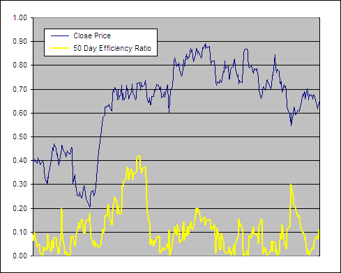
Vertical Horizontal Filter Adaptive Moving Average (VHF-AMA) – Test Results

The Adaptive Moving Average (AMA) modifies the amount of smoothing it applies to data in an attempt to adjust to the changing needs of a dynamic market.  It makes these adjustments based on the readings from a Volatility Index (VI).  Any measure of volatility or trend strength can be used, however in this article we will focus on how the AMA performs using the Vertical Horizontal Filter (VHF).

The VHF-AMA requires four user selected inputs: A Vertical Horizontal Filter period, a High – Low smoothing period range for the AMA and a power that Alpha is raised to.  With four variables there are thousands of possible combinations so we had to make some educated assumptions based on our previous tests to narrow the choices down.

In our tests on the Vertical Horizontal Filter in a VHF-VMA we revealed that VHF periods of 126, 252 and 80 produced the best results.  Because Volatility Index settings have proven to produce similar results in both the VMA and the AMA, testing these three settings should be sufficient to capture the best results.  Also they corresponded with the approximate number of trading days in standard calendar periods: 80 days = ⅓ year, 126 days = ½ year and there are 252 trading days in an average year, so:

VHF = 80, 126, 252

In previous tests we have seen that a moving average range produces the best results when it can move to as little as 4 periods or less, therefore we will test:

AMA Actual Fast Moving Average (FN) = 1, 4, 10

With the slow moving average we have consistently seen 300 produce the best results while changing this setting hasn’t usually made a big impact.  However we still ran tests through several settings:

AMA Actual Slow Moving Average (SN) = 200, 250, 300

For the Alpha Power we also tried several variables:

Alpha Power (P) = 0.5, 0.75, 1, 1.5, 2, 2.5

We tested trades going Long, using Daily data, taking End Of Day (EOD) signals~ analyzing all combinations of the above settings.

Each time the Alpha Power was adjusted the SC and FC had to be modified to account for the change but the actual FN and SN stayed the same.

For instance a SC – FC range of 1 – 24 with alpha ^ 2 has an actual FN – SN range of about 1 – 300 due to the effect of squaring alpha.  Here is a table that shows the SC – FC ranges used so that the FN – SN ranges stayed constant regardless of ‘P’:
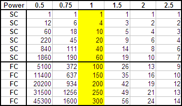
SC and FC values used to keep FN and SN constant as P was changed.

If that doesn’t make a lot of sense then please read our explanation of the Adaptive Moving Average.  A total of 162 different averages were tested and each one was run through 300 years of data across 16 different global indexes (details here).

Download A FREE Spreadsheet With Raw Data For

All 162 VHF-AMA Test Results


Vertical Horizontal Filter Adaptive Moving Average – Test Array
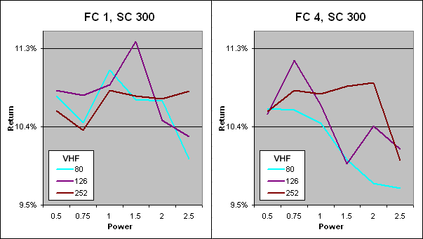
 Vertical Horizontal Filter AMA - Ann Return as Alpha Power is Changed

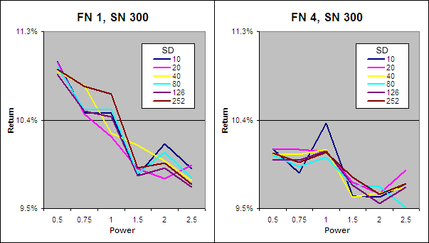
Above we have charted the annualized returns achieved from each VHF with Alpha raised to different powers along the X axis.  The chart on the left shows the results when the FN = 1 and SN = 300 while on the right FN = 4 and SN = 300.  Clearly keeping the FN at 1 is important to achieve the best returns.  A VHF period of 126 stood out as the best performer and this echoes previous tests.  Finally, when FN = 1, raising Alpha to the power of 1.5 yielded the best results.


Best Vertical Horizontal Filter Adaptive Moving Average
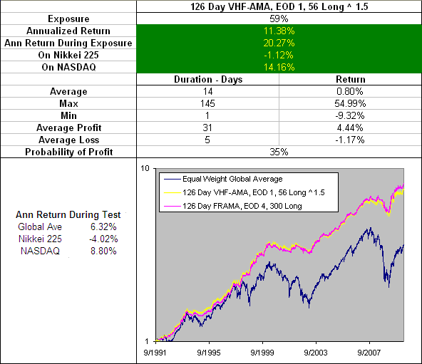
126 Day VHF-AMA, EOD 1, 56 ^ 1.5 L - Performance

Included on the above chart is the performance of the 126 Day FRAMA, EOD 4, 300 Long because so far this has been the best performing Moving Average.  The 126 Day VHF-AMA, EOD 1, 56 Long ^ 1.5 produced extremely similar results and even had the same average trade duration of 14 days.  However it did slightly underperform the FRAMA by most measures but lets take a quick look under the hood to see what makes it tick:


126 Day VHF-AMA, EOD 1, 56 ^ 1.5 – Smoothing Period Distribution
126 Day VHF-AMA, EOD 1, 56 ^ 1.5 - Smoothing Distribution

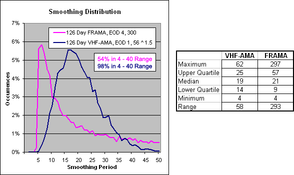
As you can see the VHF-AMA does not have nearly as much of a spread with its smoothing range as the FRAMA.  A larger range makes the FRAMA more able to adapt to different market environments.


126 Day VHF-AMA 1, 56 ^ 1.5 – Alpha Comparison

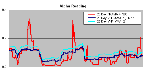
To get an idea of the readings that created these results we charted a section of the alpha for the 126 Day VHF-AMA 1, 56 ^ 1.5 and compared it to the best performing FRAMA and the best VHF-VMA to see if we could learn what makes a good volatility index for use in an AMA:.
126 Day VHF-AMA, EOD 1, 56 ^ 1.5 - Alpha Comparison

The VHF does not look as though it can change as nimbly as the FRAMA while both the AMA and VMA using a VHF look very similar.


Excel Spreadsheet

The VHF is outstanding for use in an AMA and we have build an excel spreadsheet for you to download free so you can have a play.  Simply use the flowing link and you will find it under Downloads – Technical Indicators: Adaptive Moving Average (AMA).


For more in this series see – Technical Indicator Fight for Supremacy


  • ~ An entry signal to go long for each average tested was generated with a close above that average and an exit signal was generated on each close below that moving average.  No interest was earned while in cash and no allowance has been made for transaction costs or slippage.  Trades were tested using End Of Day (EOD) signals on Daily data. Eg. Daily data with EOD signals would require the Daily price to close above a Daily Moving Average to open a long and to close below that Average to close the position.
  • We used the average annualized return of the 16 markets during the testing period.  The data used for these tests is included in the results spreadsheet and more details about our methodology can be found here.
252 Day ER-AMA, 9 – AMA Indicator Equivalent

Relative Volatility Index Adaptive Moving Average (RVI-AMA) – Test Results

The Adaptive Moving Average (AMA) modifies the amount of smoothing it applies to data in an attempt to adjust to the changing needs of a dynamic market.  It makes these adjustments based on the readings from a Volatility Index (VI).  Any measure of volatility or trend strength can be used, however in this article we will focus on how the AMA performs using the Relative Volatility Index (RVI).

The RVI-AMA requires five user selected inputs: A Standard Deviation period, a Wilder’s Smoothing period, a High – Low smoothing period range for the AMA and a power that Alpha is raised to.  With five variables there are thousands of possible combinations so we had to make some educated assumptions based on our previous tests to narrow the choices down.

In our tests on the Relative Volatility Index in a RVI-VMA we revealed that a Wilder’s Smoothing (WS) period of 14 worked the best and there is no reason to suggest that this will not also be true for a RVI-AMA so:

WS = 14

We selected the SD lengths that corresponded with the approximate number of trading days in standard calendar periods: 10 days = two weeks, 20 days = 1 month, 40 days = 2 months, 80 days = ⅓ year, 126 days = ½ year and there are 252 trading days in an average year:

SD = 10, 20, 40, 80, 126, 252

In previous tests we have seen that a moving average range produces the best results when it can move to as little as 4 periods or less, therefore we will test:

AMA Actual Fast Moving Average (FN) = 1, 4, 10

With the slow moving average we have consistently seen 300 produce the best results while changing this setting hasn’t usually made a big impact.  However we still ran tests through several settings:

AMA Actual Slow Moving Average (SN) = 100, 150, 200, 250, 300

For the Alpha Power we also tried several variables:

Alpha Power (P) = 0.5, 0.75, 1, 1.5, 2, 2.5

We tested trades going Long, using Daily data, taking End Of Day (EOD) signals~ analyzing several combinations of the above settings.

Each time the Alpha Power was adjusted the SC and FC had to be modified to account for the change but the actual FN and SN stayed the same.

For instance a SC – FC range of 1 – 24 with alpha ^ 2 has an actual FN – SN range of about 1 – 300 due to the effect of squaring alpha.  Here is a table that shows the SC – FC ranges used so that the FN – SN ranges stayed constant regardless of ‘P’:

SC and FC values used to keep FN and SN constant as P was changed.

If that doesn’t make a lot of sense then please read our explanation of the Adaptive Moving Average.  A total of 321 different averages were tested and each one was run through 300 years of data across 16 different global indexes (details here).

Download A FREE Spreadsheet With Raw Data For

All 321 RVI-AMA Test Results


Relative Volatility Index Adaptive Moving Average – Test Array

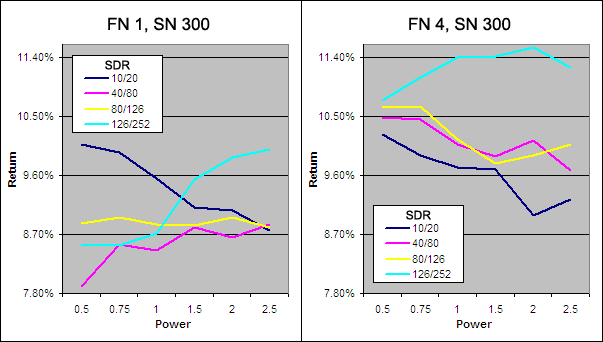
Relative Volatility Index AMA - Ann Return as Alpha Power is Changed

Above we have charted the annualized returns achieved from each RVI with Alpha raised to different powers along the X axis.  The chart on the left shows the results when the FN = 1 and SN = 300 while on the right FN = 4 and SN = 300.  Clearly keeping the FN at 1 is important to achieve the best returns.  There was no SD period that really stood out so we shall go with 126 because of how it has performed in past tests.  Finally, when FN = 1, raising Alpha to the power of 0.5 clearly yielded the best results.


Best Relative Volatility Index Adaptive Moving Average

126 Day RVI-AMA, EOD 1, 45300 ^ 0.5 (WS 14) - Performance

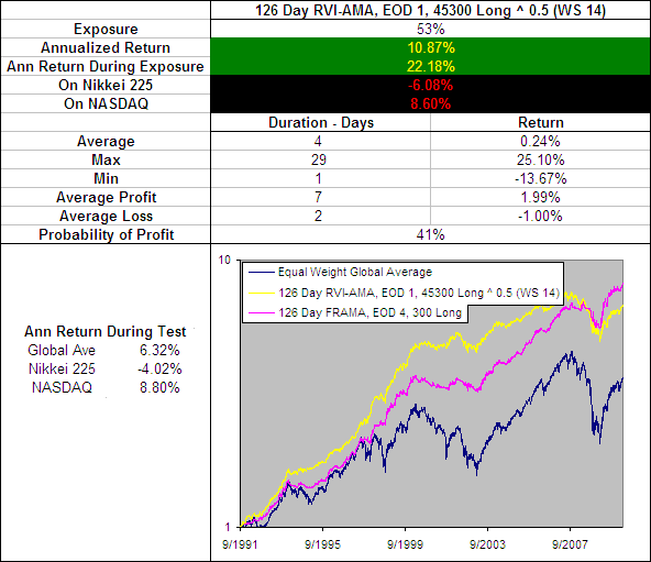
Included on the above chart is the performance of the 126 Day FRAMA, EOD 4, 300 Long because so far this has been the best performing Moving Average.  The 126 Day RVI-AMA, EOD 1, 45300 Long ^ 0.5 (WS 14) produced an extremely fast moving average with a typical trade duration of just 4 days.  This makes it unpractical for a real world application.  Add to this the fact that it underperformed the best the FRAMA and this indicator is hardly worthy of further testing.  However lets take a quick look under the hood to see what makes it tick and the causes of its weaknesses:


126 Day RVI-AMA, EOD 1, 45300 ^ 0.5 (WS 14) – Smoothing Period Distribution

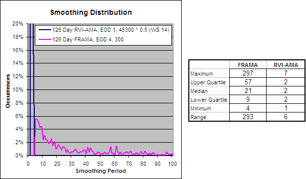
126 Day RVI-AMA, EOD 1, 45300 ^ 0.5 (WS 14) - Smoothing Distribution

Instantly you can see a big problem; there isn’t really any smoothing distribution at all from the 126 Day RVI-AMA, EOD 1, 45300 ^ 0.5 (WS 14), instead it is basically a 2 day EMA.  The far better performing FRAMA 0n the other hand has a wide spread of smoothing making on it much more adaptive to changing market conditions.


126 Day RVI-AMA 1, 45300 ^ 0.5 (WS 14) – Alpha Comparison

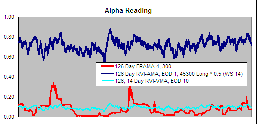
To get an idea of the readings that created these results we charted a section of the alpha for the 126 Day RVI-AMA 1, 45300 ^ 0.5 (WS 14) and compared it to the best performing FRAMA and the best RVI-VMA to see if we could learn what makes a good volatility index for use in an AMA:.

126 Day RVI-AMA, EOD 1, 45300 ^ 0.5 (WS 14) - Alpha Comparison

Higher alpha readings result in a faster average and instantly you can see the RVI-AMA has a very high Alpha compared to the best RVI-VMA and FRAMA.  Remember the RVI-AMA and the RVI-VMA both use the same volatility index but the different ways that the two modify Alpha result in a very different outcome.


Excel Spreadsheet

The RVI-AMA is not very useful but should you want to test it or another volatility index then we have build an excel spreadsheet for you to download free.  Simply use the flowing link and you will find it under Downloads – Technical Indicators: Adaptive Moving Average (AMA).


For more in this series see – Technical Indicator Fight for Supremacy


  • ~ An entry signal to go long for each average tested was generated with a close above that average and an exit signal was generated on each close below that moving average.  No interest was earned while in cash and no allowance has been made for transaction costs or slippage.  Trades were tested using End Of Day (EOD) signals on Daily data. Eg. Daily data with EOD signals would require the Daily price to close above a Daily Moving Average to open a long and to close below that Average to close the position.
  • We used the average annualized return of the 16 markets during the testing period.  The data used for these tests is included in the results spreadsheet and more details about our methodology can be found here.
252 Day ER-AMA, 9 – AMA Indicator Equivalent

Standard Deviation Ratio Adaptive Moving Average (SDR-AMA) – Test Results

The Adaptive Moving Average (AMA) modifies the amount of smoothing it applies to data in an attempt to adjust to the changing needs of a dynamic market.  It makes these adjustments based on the readings from a Volatility Index (VI).  Any measure of volatility or trend strength can be used, however in this article we will focus on how the AMA performs using the Standard Deviation Ratio (SDR).

The SDR-AMA requires five user selected inputs: SD1, SD2, a High – Low smoothing period range for the AMA and a power that Alpha is raised to.  With five variables there are thousands of possible combinations so we had to make some educated assumptions based on our previous tests to narrow the choices down.

First of all we have seen that nearly all of the performance characteristics exhibited by a VI have rung true in tests on both a VMA and an AMA.  When we tested the SDR in a VMA we found that it was best if SD1 was around half of SD2.  We also selected SD lengths that corresponded with the approximate number of trading days in standard calendar periods: 10 days = two weeks, 20 days = 1 month, 40 days = 2 months, 80 days = ⅓ year, 126 days = ½ year and there are 252 trading days in an average year:

SD1/SD2 = 10/20, 40/80, 80/126, 126/252

Second we have seen that a moving average range produces the best results when it can move to as little as 4 periods or less, therefore we will test:

AMA Actual Fast Moving Average (FN) = 1, 4

With the slow moving average we have consistently seen 300 produce the best results while changing this setting hasn’t usually made a big impact.  However we still ran tests through several settings:

AMA Actual Slow Moving Average (SN) = 100, 150, 200, 250, 300

For the Alpha Power we also tested several variables:

Alpha Power (P) = 0.5, 0.75, 1, 1.5, 2, 2.5

We tested trades going Long, using Daily data, taking End Of Day (EOD) signals~ analyzing several combinations of the above settings.

Now each time the Alpha Power was adjusted the SC and FC had to be modified to account for the change but the actual FN and SN stayed the same.

For instance a SC – FC range of 1 – 24 with alpha ^ 2 has an actual FN – SN range of about 1 – 300 due to the effect of squaring alpha.  Here is a table that shows the SC – FC ranges used so that the FN – SN ranges stayed constant regardless of ‘P’:

SC and FC values used to keep FN and SN constant as P was changed.

If that doesn’t make a lot of sense then please read our explanation of the Adaptive Moving Average.  A total of 240 different averages were tested and each one was run through 300 years of data across 16 different global indexes (details here).

Download A FREE Spreadsheet With Raw Data For

All 240 SDR-AMA Test Results


Standard Deviation Ratio Adaptive Moving Average – Test Array

Standard Deviation Ratio AMA - Ann Return as Alpha Power is Changed

Above we have charted the annualized returns achieved from each SDR with Alpha raised to different powers along the X axis.  The chart on the left shows the results when the FN = 1 and SN = 300 while on the right FN = 4 and SN = 300.  Clearly extending the FC to 4 had a positive effect and the best returns were achieved with a SDR of 126/252 where Alpha was raised to the power of 2.


Best Standard Deviation Ratio Adaptive Moving Average

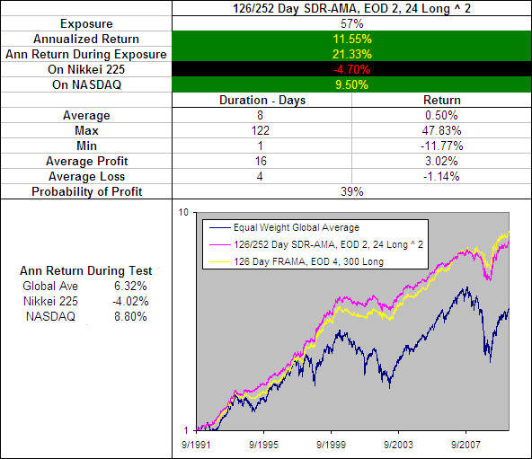
126/252 Day SDR-AMA, EOD 2, 24 Long ^ 2

Included on the above chart is the performance of the 126 Day FRAMA, EOD 4, 300 Long becuase so far this has been the best performing Moving Average.  The 126 Day SDR-AMA, EOD 2, 24 Long ^ 2 performed OK but could not best the FRAMA and has a much shorter average trade duration; just 8 days compared to 14 for the FRAMA.  For these reasons the FRAMA remains our preferred moving average and the SDR-AMA does not warrant further testing.  But lets take a quick look under the hood:


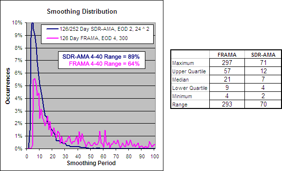
126 Day SDR-AMA, EOD 2, 24 ^ 2 – Smoothing Period Distribution

126/252 Day SDR-AMA, EOD 2, 24 ^ 2 Smoothing Period Distribution

The smoothing distribution of the 126 Day SDR-AMA, EOD 2, 24 ^ 2 is much more localised around the 4 – 20 range than the FRAMA which explains the shorter trade duration.  The FRAMA on the other hand allows the average to move much slower at times, presumably when the trend is weak.


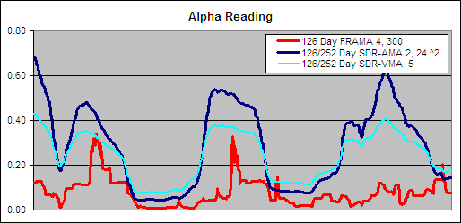
126 Day SDR-AMA 2, 24 ^ 2 – Alpha Comparison

To get an idea of the readings that created these results we charted a section of the alpha for the 126 Day SDR-AMA 2, 24 ^ 2 and compared it to the best performing FRAMA and the best SDR-VMA to see if there were any similarities that would reveal what makes a good volatility index:.

126/252 Day SDR-AMA, EOD 2, 24 ^ 2 - Alpha Comparison

Remember higher alpha readings result in a faster average.  The SDR-AMA and the SDR-VMA are clearly both much faster than the FRAMA.  However the SDR-AMA does slightly outperform the SDR-VMA and notice that the SDR-AMA’s Alpha moves through a greater range from high to low.  This greater ‘adaptability’ is likely to have been a key factor in its better performance.


Excel Spreadsheet

Want to use this indicator?  Get a free Excel spreadsheet at the flowing link under Downloads – Technical Indicators: Adaptive Moving Average (AMA).  It will automatically adjust to your choice of many different VIs including the Standard Deviation Ratio used in this article.


For more in this series see – Technical Indicator Fight for Supremacy


  • ~ An entry signal to go long for each average tested was generated with a close above that average and an exit signal was generated on each close below that moving average.  No interest was earned while in cash and no allowance has been made for transaction costs or slippage.  Trades were tested using End Of Day (EOD) signals on Daily data. Eg. Daily data with EOD signals would require the Daily price to close above a Daily Moving Average to open a long and to close below that Average to close the position.
  • We used the average annualized return of the 16 markets during the testing period.  The data used for these tests is included in the results spreadsheet and more details about our methodology can be found here.
252 Day ER-AMA, 9 – AMA Indicator Equivalent

Fractal Dimension Adaptive Moving Average (D-AMA) – Test Results

The Adaptive Moving Average (AMA) modifies the amount of smoothing it applies to data in an attempt to adjust to the changing needs of a dynamic market.  It makes these adjustments based on the readings from a Volatility Index (VI).  Any measure of volatility or trend strength can be used, however in this article we will focus on how the AMA performs using the Fractal Dimension (D).  This is the VI used in the FRAMA which has so far been the best performing Moving Average we have tested.

We did have to make one slight modification to the Fractal Dimension however.  The Volatility index in an AMA needs to shift through a 0 – 1 range where higher readings indicate a stronger trend.  The Fractal Dimension shifts through a 1 – 2 range where lower readings indicate a stronger trend.  Therefore we shall use = ABS(D – 2).

The D-AMA requires four user selected inputs: A Fractal Dimension Period, a High – Low smoothing period range for the AMA and a power that Alpha is raised to.  We tested trades going Long, using Daily data, taking End Of Day (EOD) and End of Week (EOW) signals~ analyzing combinations of:

D = 40, 80, 126, 252

Alpha Power (P) = 0.5, 0.75, 1, 1.5, 2, 2.5

AMA Actual Fast Moving Average (FN) = 1, 4, 10, 20, 40, 60

AMA Actual Slow Moving Average (SN) = 100, 150, 200, 250, 300

The D lengths were selected due to the fact that they correspond with the approximate number of trading days in standard calendar periods: 40 days = 2 months, 80 days = ⅓ year, 126 days = ½ year and there are 252 trading days in an average year.  In many of out past tests we have also tested VI lengths of 10 and 20 days, however these setting have always failed to yield the best results so we felt that it would be safe to omit them from this set of tests.

The AMA ranges were selected because they should capture the best results based on what we know from previous research into moving averages.  Each time the Alpha Power was adjusted the SC and FC had to be modified to account for the change but the actual FN and SN stayed the same.

For instance a SC – FC range of 1 – 24 with alpha ^ 2 has an actual FN – SN range of 1 – 300 due to the effect of squaring alpha.  Here is a table that shows the SC – FC ranges used so that the FN – SN ranges stayed constant regardless of ‘P’:

SC and FC values used to keep FN and SN constant as P was changed.

If that doesn’t make a lot of sense then please read our explanation of the Adaptive Moving Average.  A total of 960 different averages were tested and each one was run through 300 years of data across 16 different global indexes (details here).

Download A FREE Spreadsheet With Raw Data For

All 960 D-AMA Test Results


Fractal Dimension Adaptive Moving Average – Modifying Alpha by Raising to a Power

Kaufman had a theory that by squaring Alpha and thus causing the AMA to slow rapidly when the data lacked a strong trend he would achieve better results.  When we tested this theory on the ER-AMA we found it to be false but with a different VI we may reach a different conclusion.  So lets look at the affect of raising Alpha to different powers:

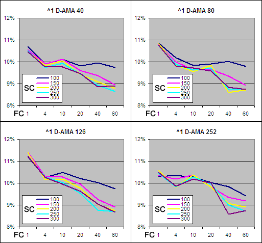
Fractal Dimension – AMA, Alpha to the Power of  1 – Annualized Return

Fractal Dimension - AMA ^ 1 - Annualized Return

With Alpha ^1 there is no modification to Alpha at all.  Clearly as the FC is increased the returns decline and as the FC gets higher the change in SC has more impact.  Generally it appears as though a SC of 100 is best on a D-AMA with an unmodified Alpha.   ER lengths of 80 and 126 yielded the best returns, this finding is similar to that of our previous tests on other ‘intelligent’ moving averages.

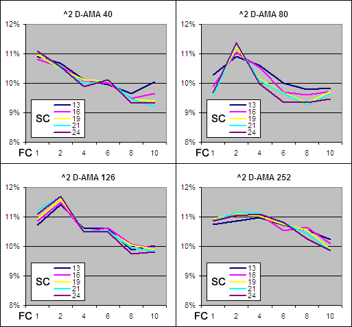
Fractal Dimension – AMA to the Power of  2 – Annualized Return

Fractal Dimension - AMA ^ 2 - Annualized Return

By raising Alpha to the power of 2, returns at almost all the data points increased which is just the opposite of what we experienced when testing the ER-AMA.  This shows that Kaufman’s theory of rapidly slowing the AMA during times where a trend is lacking had merit but is dependent on the VI being used.

The best results again came from ER lengths of 80 and 126 although an ER length of 40 did produce some notable returns.  Changing the SC did not have as much of an effect with Alpha ^2 compared to Alpha ^ 1 however a SC of 24 (SN equivalent of 300) and a short FC tends to produce the best results.  So lets rework the charts to focus on what we now know works best:

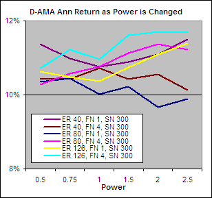
D-AMA Annualized Return with Alpha to Different Powers

Now we are only looking at ER periods of 40, 80 and 126 with a FN of 1 and 4 and a SN of 300.  Each data point plots the change in returns with Alpha raised to different powers.  As you can see, the best returns resulted from an ER period of 126 with alpha raised to the power of 2.  Therefore when using the Fractal Dimension in an Adaptive Moving average you are best to square alpha as suggested in the original formula..


Best EOD Fractal Dimension Adaptive Moving Average

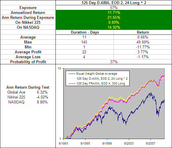
126 Day D-AMA, EOD 2, 24 Long ^ 2

I have included on the above chart the performance of the 126 Day FRAMA, EOD 4, 300 Long becuase so far this has been the best performing Moving Average.  The 126 Day D-AMA, EOD 2, 24 Long ^ 2 put up a good fight against the FRAMA but ultimately underperformed by most measures to a small degree.  On the Short side, the the D-AMA also underperformed slightly.


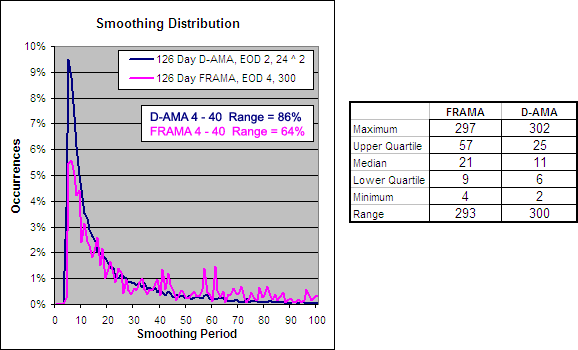
126 Day D-AMA, EOD 2, 24 ^ 2 – Smoothing Period Distribution

126 Day D-AMA 2, 24 ^ 2 Smoothing Period Distribution

Looking at the smoothing distribution you can see the 126 Day D-AMA, EOD 2, 24 ^ 2 is very similar to that of the 126 Day FRAMA, EOD 4, 300 but the FRAMA allows the average to slow down more often.


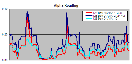
126 Day D-AMA 2, 24 ^ 2 – Alpha Comparison

To get an idea of the readings that created these results we charted a section of the alpha for the 126 Day D-AMA 2, 24 ^ 2 and compared it to the best performing FRAMA and the best D-VMA to see if there were any similarities that would reveal what makes a good volatility index:.

126 Day D-AMA 2, 24 ^ 2 - Alpha Comparison

You can clearly see that all three use the same VI, the only difference is how they manipulate Alpha.  Remember, higher readings result in a faster average so the D-AMA is obviously the fastest of the three while the FRAMA appears to shift through the widest range.


Best EOW Fractal Dimension Adaptive Moving Average

There are times when an average with a longer trade duration better suits ones needs so we also ran the tests looking for the best average using EOW signals, here is the one that came out trumps:

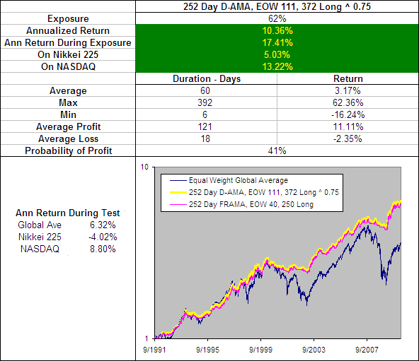
252 Day D-AMA. EOW 111, 372 Long ^ 0.75

We have included on the above chart the performance of the 252 Day FRAMA, EOW 40, 250 Long becuase so far this has been the best performing EOW Moving Average.  The 252 Day D-AMA, EOW 111, 372 Long ^0.75 is almost identical to the FRAMA but does outperform it by a fraction.  They are so similar in fact that they may as well be the same average.  Performance on the short side tells the same story.


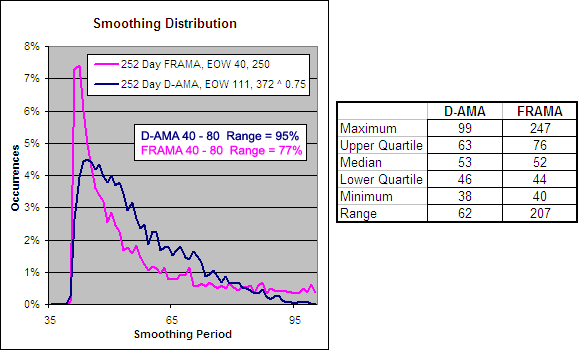
252 Day D-AMA, EOW 111, 372 ^ 0.75 – Smoothing Period Distribution

252 Day D-AMA, EOW 111, 372 ^ 0.75 - Smoothing Period Distribution

The smoothing distribution for the 252 Day D-AMA 111, 372 ^ 0.75 has a smaller range than that of the 252 Day FRAMA 40, 250 but the median, lower quartile and minimum are almost identical.  You can view an Alpha Comparison Here.


Conclusion

In our tests on the ER-AMA we came to the conclusion that the squaring of alpha as suggested in the standard AMA formula was actually detrimental to performance.  However when using the Fractal Dimension as the VI, squaring Alpha was beneficial.  Therefore the best Power to use in manipulating alpha varies depending on the VI in use.

Overall the D-AMA produced results that were near identical to that of the FRAMA but the D-AMA is a slightly faster average.  The best performing EOD D-AMA was the 126 Day ER-AMA, EOD 2, 26 ^ 2 while the best EOW or ‘slower’ moving average was the 252 Day D-AMA, EOW 111, 372 ^ 0.75.

It is very difficult to pick between the FRAMA and the D-AMA but becuase the FRAMA offers a slightly longer trade duration it the best Moving Average we have tested so far.

Want to use this indicator?  Get a free Excel spreadsheet at the flowing link under Downloads – Technical Indicators: Adaptive Moving Average (AMA).  It will automatically adjust to your choice of many different VIs including the Fractal Dimension used in this article.


For more in this series see – Technical Indicator Fight for Supremacy


  • ~ An entry signal to go long (or exit signal to cover a short) for each average tested was generated with a close above that average and an exit signal (or entry signal to go short) was generated on each close below that moving average.  No interest was earned while in cash and no allowance has been made for transaction costs or slippage.  Trades were tested using End Of Day (EOD) and End Of Week (EOW) signals on Daily data. Eg. Daily data with an EOW signal would require the Week to finish above a Daily Moving Average to open a long or close a short while Daily data with EOD signals would require the Daily price to close above a Daily Moving Average to open a long or close a short and vice versa.
  • We used the average annualized return of the 16 markets during the testing period.  The data used for these tests is included in the results spreadsheet and more details about our methodology can be found here.
252 Day ER-AMA, 9 – AMA Indicator Equivalent

Efficiency Ratio Adaptive Moving Average (ER-AMA) – Test Results

The Adaptive Moving Average (AMA) modifies the amount of smoothing it applies to data in an attempt to adjust to the changing needs of a dynamic market.  It makes these adjustments based on the readings from a Volatility Index (VI). Any measure of volatility or trend strength can be used, however in this article we will focus on how the AMA performs using an Efficiency Ratio (ER).  This is the VI that Perry Kaufman used when he presented the AMA in his book Smarter Trading (1995).

The ER-AMA requires four user selected inputs: An Efficiency Ratio Period, a High – Low smoothing period range for the AMA and a power that Alpha is raised to.  We tested trades going Long, using Daily data, taking End Of Day (EOD) and End of Week (EOW) signals~ analyzing combinations of:

ER = 10, 20, 40, 80, 126, 252

Alpha Power (P) = 0.5, 0.75, 1, 1.5, 2, 2.5

AMA Actual Fast Moving Average (FN) = 1, 4, 10, 20, 40, 60

AMA Actual Slow Moving Average (SN) = 100, 150, 200, 250, 300

The ER lengths were selected due to the fact that they correspond with the approximate number of trading days in standard calendar periods: 10 days = 2 weeks, 20 days = 1 month, 40 days = 2 months, 80 days = ⅓ year, 126 days = ½ year and there are 252 trading days in an average year.

The AMA ranges were selected because they should capture the best results based on what we know from previous research into moving averages.  Each time the Alpha Power was adjusted the SC and FC had to be modified to account for the change but the actual FN and SN stayed the same.

For instance a SC – FC range of 1 – 24 with alpha ^ 2 has an actual FN – SN range of 1 – 300 due to the effect of squaring alpha.  Here is a table that shows the SC – FC ranges used so that the FN – SN ranges stayed constant regardless of ‘P’:

SC and FC values used to keep FN and SN constant as P was changed.

If that doesn’t make a lot of sense then please read our explanation of the Adaptive Moving Average.  A total of 1020 different averages were tested and each one was run through 300 years of data across 16 different global indexes (details here).

Download A FREE Spreadsheet With Raw Data For

All 1020 ER-AMA Test Results


ER Adaptive Moving Average – Modifying Alpha by Raising to a Power

Kaufman had a theory that by squaring Alpha and thus causing the AMA to slow rapidly when the data lacked a strong trend he would achieve better results.  Here we will put this theory to the test and be looking at the affect of raising Alpha to different powers:

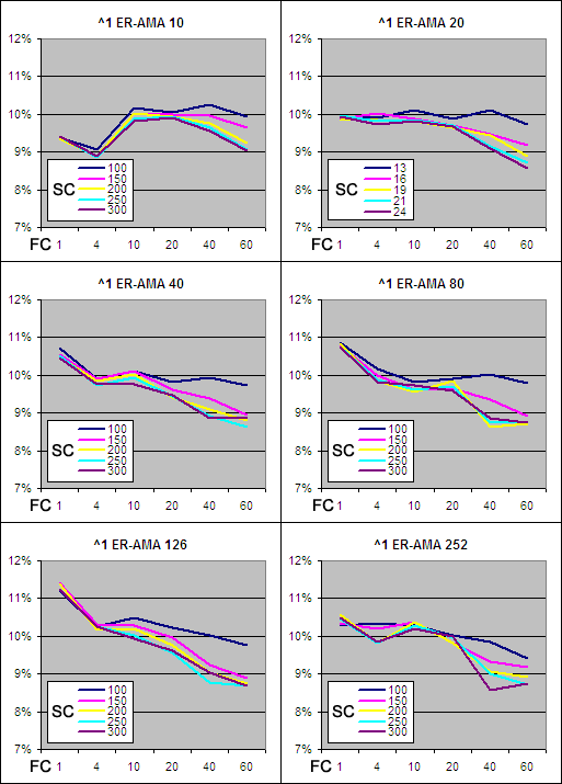
Efficiency Ratio – AMA, Alpha to the Power of  1 – Annualized Return

Efficiency Ratio - AMA ^ 1 - Annualized Return

With Alpha ^1 there is no modification to alpha at all and the results are impressive.  It can be said that in most cases as the FC increased the returns declined while changing the SC did not have much of an impact.  ER lengths of 80 and 126 yielded the best returns, this finding is similar to that of our previous tests on other ‘intelligent’ moving averages.

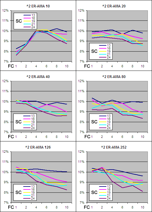
Efficiency Ratio – AMA to the Power of  2 – Annualized Return

Efficiency Ratio - AMA ^ 2 - Annualized Return

By raising Alpha to the power of 2 the returns drop almost across the board which immediately brings into question the need to include this function in the AMA formula and what would happen if we used a power below 1?  It would appear as though the ER length needs to be at least 40 to be of value in this context with the best results again coming from ER lengths of 80 and 126.  Clearly the FC is best when kept short so lets rework the charts to focus on what we now know works best:

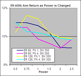
ER-AMA Annualized Return with Alpha to Different Powers

Now we are only looking at ER periods of 80 and 126 with a FN of 1 and 4 and a SN of 300.  Each data point plots the change in returns with Alpha raised to different powers.  As you can see, the best returns resulted from an ER period of 126 with alpha raised to the power of 0.75.  As the Power was increased beyond this point, the returns decreased almost across the board.  Therefore when using an Efficiency Ratio in an Adaptive Moving average you definitely should not square alpha as suggested in the original formula..


Best EOD Efficiency Ratio Adaptive Moving Average

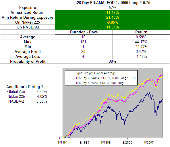
126 Day ER-AMA EOD 1, 1600 Long ^ 0.75

We have included on the above chart the performance of the 126 Day FRAMA, EOD 4, 300 Long becuase so far this has been the best performing Moving Average.  The 126 Day ER-AMA, EOD 1, 1600 Long ^ 0.75 actually outperformed the best FRAMA up until 2008 when the market had a big pull back.  As a result, over the full term of the test the FRAMA did perform slightly better.  Also the FRAMA has a few added benefits such as turning a profit on the bear ravaged Nikkei 225 and having a 40% longer average trade duration (14 vs 10 Days).

On the Short side, the the ER-AMA also underperformed over the full term but again outperformed until 2008.  This makes it very difficult to pick which moving average is the better of the two.  But because our personal preference leans towards a longer trade duration we will stick with the FRAMA as being the best moving average we have found so far.  (See the results on the short side)


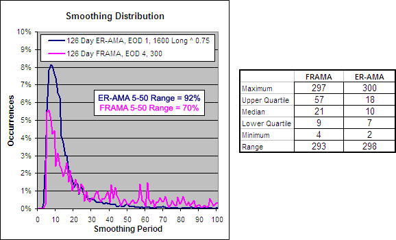
126 Day ER-AMA, EOD 1, 1600 ^ 0.75 – Smoothing Period Distribution

126 Day ER-AMA, EOD 1, 1600 ^ 0.75 - Smoothing Period Distribution

Looking at the smoothing distribution you can see the 126 Day ER-AMA, EOD 1, 1600 ^ 0.75 is quite similar to that of the 126 Day FRAMA, EOD 4, 300 but the FRAMA spends more time as a slow average which explains the longer trade duration.


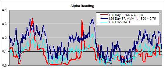
126 Day ER-AMA, 1, 1600 ^ 0.75 – Alpha Comparison

To get an idea of the readings that created these results we charted a section of the alpha for the 126 Day ER-AMA, 1, 1600 ^ 0.75 and compared it to the best performing FRAMA and the best ER-VMA to see if there were any similarities that would reveal what makes a good volatility index:.

126 Day ER-AMA, 1, 1600, ^ 0.75 - Alpha Comparison

Because the ER-AMA and the ER-VMA both use the same volatility index, obviously their Alpha is identical apart from the slight modifications caused by the separate method of manipulating alpha.  Remember, the higher the Alpha the faster the resulting average so you can see why the best ER-AMA was faster moving than the best ER-VMA.  The Alpha patterns of the best FRAMA and best ER-AMA do have strong similarities but notice how the FRAMA is far less volatile.  It is always preferable to work with indicators that generate clean readings with low levels of noise assuming they still produce good results.


Best EOW Efficiency Ratio Adaptive Moving Average

There are times when an average with a longer trade duration better suits ones needs so we also ran the tests looking for the best average using EOW signals:

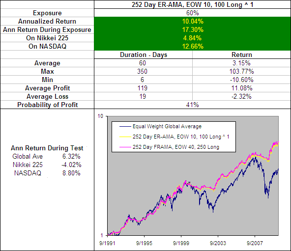
252 Day ER-AMA, EOW 10, 100 Long ^ 1

We have included on the above chart the performance of the 252 Day FRAMA, EOW 40, 250 Long becuase so far this has been the best performing EOW Moving Average.  The 252 Day ER-AMA, EOW 10, 100 Long ^1 underperforms by a fraction in most measures and while almost identical to the FRAMA it certainly is not superior.  Performance on the short side tells the same story.


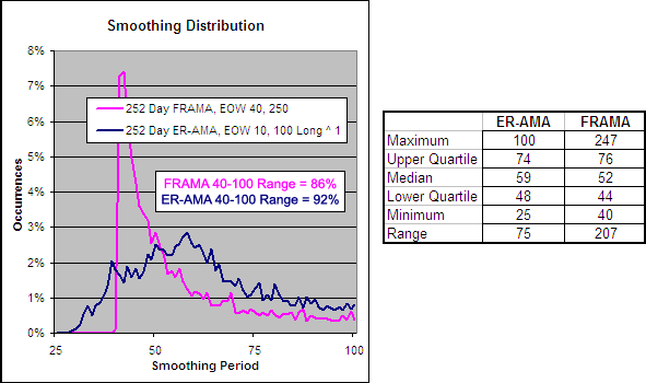
252 Day ER-AMA, EOW 10, 100 ^ 1 – Smoothing Period Distribution

252 Day ER-AMA, EOW 10, 100 ^ 1 - Smoothing Period Distribution

Looking at the smoothing distribution for the 252 Day ER-AMA 10, 100 ^ 1 you can see that it is far faster than the 252 Day FRAMA 40, 250 and has a more limited range despite the median, upper and lower quartiles being almost identical.


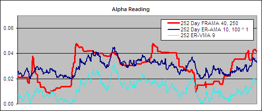
252 Day ER-AMA 10, 100 ^ 1 – Alpha Comparison

252 Day ER-AMA 10, 100 ^ 1 - Alpha ComparisonWe have included on this chart the best EOW FRAMA and EOW ER-VMA.  The ER-VMA and ER-AMA use the same volatility index but the 252 Day ER-AMA 10, 100 ^1 results in a higher Alpha which explains the faster average.  The Alpha for the FRAMA and the AMA does stay in a similar zone but the FRAMA is far less volatile which is preferable.


Conclusion

In the standard formula for the AMA, alpha is squared to force the average to slow rapidly during times when there is a lack of trend.  When using an Efficiency Ratio as the Volatility Index (which is most commonly used VI in an AMA) we have clearly shown that squaring Alpha has a detrimental effect on returns.  We suggest instead not modifying alpha at all or raising it to the power of 0.75

Overall the ER produced some impressive returns during out tests as the VI in an AMA as it did when we used in a VMA.  The best performing EOD ER-AMA was a 126 Day ER-AMA, EOD 1, 1600 Long ^ 0.75 which did show periods of out performance over our current best performing MA the 126 Day FRAMA, EOD 4, 300 Long.  However due to a longer trade duration we still rate the FRAMA as superior.

When it comes to an EOW or ‘slower’ moving average the 252 Day ER-AMA, EOW 10, 100 ^ 1 is almost identical to our current best ‘slow’ MA the 252 Day FRAMA, EOW 40, 250 Long but certainly does not offer any benefits.

Both the Efficiency Ratio and the Adaptive Moving Average have proven themselves against some formidable competition but based on our findings so far the FRAMA still remains slightly superior.

Want to use this indicator? Get a free Excel spreadsheet at the flowing link under Downloads – Technical Indicators: Adaptive Moving Average (AMA).  It will automatically adjust to your choice of many different VIs including the Efficiency Ratio used in this article.


For more in this series see – Technical Indicator Fight for Supremacy


  • ~ An entry signal to go long (or exit signal to cover a short) for each average tested was generated with a close above that average and an exit signal (or entry signal to go short) was generated on each close below that moving average.  No interest was earned while in cash and no allowance has been made for transaction costs or slippage.  Trades were tested using End Of Day (EOD) and End Of Week (EOW) signals on Daily data. Eg. Daily data with an EOW signal would require the Week to finish above a Daily Moving Average to open a long or close a short while Daily data with EOD signals would require the Daily price to close above a Daily Moving Average to open a long or close a short and vice versa.
  • We used the average annualized return of the 16 markets during the testing period.  The data used for these tests is included in the results spreadsheet and more details about our methodology can be found here.
252 Day ER-AMA, 9 – AMA Indicator Equivalent

Adaptive Moving Average (AMA) aka Kaufman Adaptive Moving Average (KAMA)

The Adaptive Moving Average (AMA) aka Kaufman Adaptive Moving Average (KAMA) was created by Perry Kaufman and first presented in his book Smarter Trading (1995).  This moving average offered a significant advantage over previous attempts at ‘intelligent’ averages because it allowed the user greater control.

The Variable Moving Average – VMA (1992) for instance offered no upper or lower limit to its smoothing period.  The AMA on the other hand allowed the user to define the range across which they desired the smoothing to be spread.

It follows the same theory as the VMA in that depending on the market environment there will be different amounts of noise and therefore a different moving average speed will be required to achieve the most profitable results.  In a strongly trending market for instance, the noise levels are low and a faster moving average should produce the best results.  Conversely in a crab or sideways market the noise levels are very high and a slower average is likely to be better suited.

.

How to Calculate an Adaptive Moving Average

.

It starts with the Close price.

AMA(1) = Close

After that AMA is calculated according to the following formula:

AMA = AMA(1) + α * (Close – AMA(1))

You will notice that this is the same as the formula for an Exponential Moving Average (EMA):

EMA = EMA(1) + α * (Close – EMA(1))

But Alpha in an EMA is α = 2 / (N + 1) so it remains constant while for an AMA the Alpha is adaptive:

α = [(VI * (FC – SC)) + SC] ²

Where:

VI = Users choice of a measure of volatility or trend strength, Kaufman suggested his Efficiency Ratio (ER).

SC = 2 / (SN + 1)

SN = Your choice of a Slow moving average > FN

FC = 2 / (FN + 1)

FN = Your choice of a Slow moving average < SN

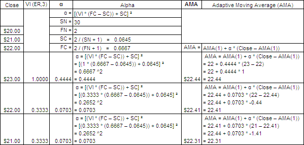
Here is an example of a 3 period AMA with a 3 period Efficiency Ratio (ER) as the VI:

.

Adaptive Moving Average Formula.

How Squaring Alpha affects the AMA Smoothing Range

.

Kaufman suggest that his AMA have a FC of 2 and a SC of 30 which would lead one to assume that the adaptive smoothing would be in the 2 – 30 range but you would be wrong because the alpha is squared.  For example, lets set the VI to zero so we can reveal the slowest possible average:

.

AMA Alpha Calculations.

Now to reveal the EMA smoothing period ‘N’ from alpha:

N (EMA) = (2 – α) / α
N (EMA) = (2 – 0.0042) / 0.0042
N (EMA) = 480

So in reality an AMA with a SN of 30 where alpha is raised to the power of 2 can actually move as slowly as a 480 day EMA.  Now to me that is not very user friendly; entering a parameter of 30 that results in a smoothing period of 480.  So I use the following formula for SC and FC instead:

SC = α(1)^(1/P)

Where:

α(1) = 2 / (SN+1)

P = Power that alpha is raised to (usually 2)

SN = Your choice of a Slow moving average > FN

Now SN will be the actual resulting slowest moving average even if you change the power that alpha is raised to.  I also use the same process for FN and FC.  Lets look again at Alpha with the VI set to zero, the FN at 2 and the SN at 480:

.

AMA New Alpha Calculations.

Now when we reveal the EMA smoothing period ‘N’ from alpha it should equal our user defined 480:

N (EMA) = (2 – α) / α
N (EMA) = (2 – 0.0042) / 0.0042
N (EMA) = 480

.

A closer look at the affect of Squaring Alpha

.

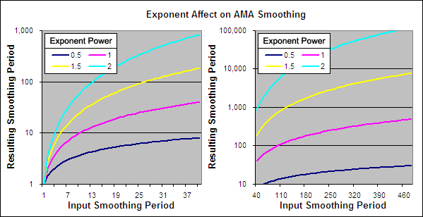
Understanding the affect of squaring alpha is very important as the chart below illustrates:

.

AMA Exponent Affect on Smoothing

.

As you can see above, an input smoothing period of 300 with alpha squared results in an actual smoothing period of over 45,300 which is totally useless.  However this is a setting that one could easily use without a proper understanding of how the AMA works.  In our testing we will be trying the AMA with alpha raised to powers other that 2 so some other examples have also been plotted on the chart above.

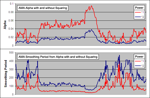
Below we look at the affect on alpha and the smoothing resulting from an AMA with the Efficiency Ratio taken directly into alpha (^1) or being squared (^2):

.

AMA - Alpha and Smoothing with and without Squaring

.

We used our modified AMA formula for the above charts so that the actual FN and SN were identically matched despite modifications to alpha.  As you can see, squaring alpha results in not just a slower AMA overall but one that is much faster to slow down when the alpha decreases.  Kaufman obviously wanted the AMA to very rapidly slow when the data lacked a trend.  This affect is similar to that of increasing the constant ‘N’ in the Variable Moving Average.

.

Is the AMA a Good Indicator?

.

As part of the ‘Technical Indicator Fight for Supremacy‘ we will be putting the AMA against several different types of moving averages and will test several different Volatility Indexes as components including:

We will also be testing the assumption that squaring alpha was a good idea and will try raising it to several different powers.

Can you think of any other worthwhile tests?  Please let us know in the comments section at the bottom.

.

Adaptive Moving Average Excel File

.

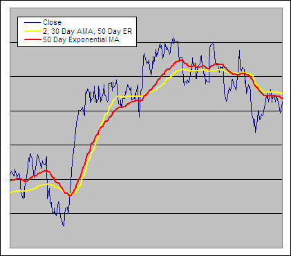
I have put together an Excel Spreadsheet containing the Adaptive Moving Average and made it available for FREE download.  It contains a ‘basic’ version that shows all the working and a ‘fancy’ one that will automatically adjust to the length as well as the Volatility Index you specify.  Find it at the following link near the bottom of the page under Downloads – Technical Indicators: Adaptive Moving Average (AMA)

.

Adaptive Moving Average Example, VI = 50 Day Efficiency Ratio

.

Kaufman Adaptive Moving Average vs EMA - Example

Kaufman’s Efficiency Ratio (ER)

The Efficiency Ratio (ER) was first presented by Perry Kaufman in his 1995 book ‘Smarter Trading‘.  It is calculated by dividing the price change over a period by the absolute sum of the price movements that occurred to achieve that change.  The resulting ratio ranges between 0 and 1 with higher values representing a more efficient or trending market.

The ER is actually very similar to the Chande Momentum Oscillator (CMO) presented by Tushar S. Chande in ‘The New Technical Trader‘ (1994).  The difference is that the CMO takes into account for market direction but if you take the absolute CMO and divide by 100 you you get the Efficiency Ratio.

A measure of a trends strength can be very useful as some strategies work best on a trending market and some in a range bound market.  Likewise different moving average lengths will perform better depending on the market type at that time.

Kaufman originally intended the Efficiency Ratio for use in his Adaptive Moving Average (KAMA).  But in addition to the KAMA, as part of the Technical Indicator Fight for Supremacy we will be testing it as a component in a Variable Moving Average and an Indicator Weighted Moving Average.

.

How To Calculate the Efficiency Ratio

.

ER = Direction / Volatility

Where:

Direction = ABS (Close – Close[n])

Volatility = n ∑ (ABS(Close – Close[1]))

n = The efficiency ratio period.

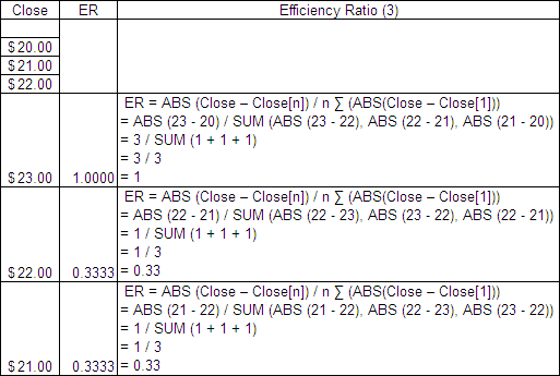
Here is an example of a 3 period ER:

.

Efficiency Ratio Formula

.

Efficiency Ratio Excel File

.

I have put together an Excel Spreadsheet containing the Kaufman’s Efficiency Ratio and made it available for FREE download.  It contains a ‘basic’ version displaying the example above and a ‘fancy’ one that will automatically adjust to the length you specify.  Find it at the following link near the bottom of the page under Downloads – Technical Indicators: Efficiency Ratio (ER).

.

Test Results

.
As part of the ‘Technical Indicator Fight for Supremacy‘ We have tested/will test the Efficiency Ratio as a component in several technical indicators:

  • Efficiency Ratio Variable Moving Average (ER-VMA) – CompletedResults
  • Efficiency Ratio Adaptive Moving Average (ER-AMA) – CompletedResults
  • Efficiency Ratio Log Normal Adaptive Moving Average (ER-LAMA)
  • Efficiency Ratio Weighted Moving Average (ER-WMA)

We will also test the ER as a filter, only taking trades when it indicates a strong trend.

.

Efficiency Ratio Example

.

Efficiency Ratio Example